A new way to extract climate signals from weather noise: Seasonal delay

via David M. Barnett

summary of Global warming as a problem of system response theory

Weather noise problem—how much warmer?

Changes in weather can cause temperatures to vary from day to day by as much as 20°C. The coldest day in mid-summer can be colder than the warmest day in mid-winter. That’s the weather. However, we all know the difference between summer and winter, and summer days are usually warmer than winter days. That is our experience of climate.

It is said that the climate has warmed by about one degree in the last 200 years. That’s a very small number so extracting from everyday noise can be an order of magnitude larger. How can one reliably extract that small secular temperature trend? Even thermometer measurements at a single site can be perturbed by global non-climate factors such as increasing urbanization or even the growth or removal of a row of trees.

Noise problem from warming—is it CO₂?

Many people think that CO₂, added to the atmosphere by burning fossil fuels since the industrial revolution, has increased the effective thermal resistance between the earth’s surface and outer space—”greenhouse warming”— forced to increase the temperature to compensate. But how to separate this “greenhouse” hypothesis from other possible contributing causes such as changes in land use or changes in sunlight? THAT’S RIGHT initial Modeling the climate system is impractical due to the large range of important spatial and temporal scales. How to extract the allocation signal from parametric noise?

Signal processing with carrier

Since the invention of the magnetic tape recorder, signal engineers have known that it is much easier to extract the desired signal from the noise if the high frequency carrier modulated signal is known.

As it happens, the seasonal variation caused by the tilt of the earth’s axis and the earth’s orbit around the sun has a known one-year period, and the excitation of the sun at any given position also has a known cycle. The climate system processes this “carrier” signal input and produces a measurable temperature output. For example, daily temperature measurements have been recorded at one site in Central England for more than two centuries. Time series available from BADC in the UK.

Climate signal

So what signal can we extract with one year period? Figure Figure 1 shows the cosine of the 1-year period in line with the 4-year block from 1772 to 1776. The blue cosine curve is the climate signal while the black curve is the daily weather noise. Not surprisingly, the coldest time of year, by climate, occurs in the second half of January. However, daily weather can vary greatly. For example, at the end of January 1773, there was an unseasonal warmth with average daily temperatures as high as 9°C, even though this was the end of the “little ice age”.

Figure first: Least squares cosine fit over a one-year period for average daily temperature data over a block of four years

Seasonal lag and climate change

I’ve always been intrigued by the fact that the shortest day of the year is around December 20th, while the coldest is usually late January. The difference is the seasonal delay. In the case of 1772 to 1776, the coldest day (according to climate) was 19.5 days in January. That represents a lag of about 30 days, roughly in radians.

Why do the seasons lag behind the length cycle of daylight? The short answer is that the oceans store heat. It is similar to the electric RC filter (see Figure 2) where C is the ocean’s ability to store heat and R is the effective resistance to heat escaping into space. The larger R or C, the longer the phase delay.

Now comes the magic. CO . gas₂ the “greenhouse” hypothesis is the addition of CO₂ increase the effective thermistor, R. In that case, the seasonal delay must increase with CO₂. The CR filter theory also predicts that the difference between summer and winter will also increase, if thermistor is the sole cause of the increase in hysteresis.

How the seasonal lag changed between 1772 and 2005 in Central England

The daily mean temperature time series for Central England is broken down into 4-year blocks. A cosine climate curve, with a period of one year, is fitted for each block (as in Figure 1 for example). The parameters for each block are Temperature Amplitude (i.e. the half temperature change from summer to winter), temperature period (expressed as days in January of the minimum climatic temperature), and Average temperature for the block. These three parameters were plotted on a graph with a horizontal axis covering the years 1772 to 2005.

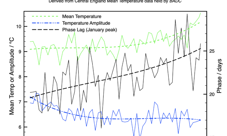
There is considerable variation in the parameters from the 4-year block to the 4-year block. Therefore, I have provided an “eye guide” to the trends in the form of least squares cubic curves that fit each parameter series. The results are summarized in Figure 3.

Figure 3: Phase lags (January days), temperature amplitudes, and average temperatures of 4-year blocks are plotted for the years 1772 to 2005, along with cubic trendlines that fit the data.

Discussing temperature trends in Central England

First consider the seasonal lag. Latency can vary quite a bit over a short period of time. However, there seems to be a long-term trend for the coldest period, from about January 20, 1800 to about January 25, 2005.

Note that although I’m expressing phase by coldest period, the fit to the data will be dominated by what happens in spring and fall when temperatures change fastest from this week to another week. Thus, while phase conformance implies the coldest climate around January 20, it could easily be followed by an “off-season” warm wave (as happened in 1773—see Figure first).

The cold depth at 20 January 1800 was 31 days later (approximately π/6 radians) than on 20 December 1799 (the shortest day). 200 years later, the lag seems to have increased to about 36 days (approximately π/5 radians) in 2004. That is a clear increase of about 5 days (approximately π/30 radians) over 200 years.

If the data can be modeled by Figure 2, the phase delay trend is consistent with the combination of an increasing “insulation” effect, R, and a storage effect, C.

Can the phase delay be attributed only to the increase in insulation?

Let us consider the hypothesis that the phase delay is purely due to increased insulation and that the input flux amplitude, J, remains constant.

From 1772 to about 1870, the temperature range between summer and winter tended to decrease gradually from about 7.2°C to about 6.4°C. It was more or less unchanged after 1870. Total CO₂ hypothesis will predict the temperature amplitude increase. In fact, the decline in the early period can’t match assuming constant input throughput, J.

It is surprising that fitting the temperature amplitude history requires J to downfall between 1772 and 1870.

The contribution of changes in R to seasonal latency variation is about 30%, while storage, C, must contribute the rest. One can speculate that the increase in C is due to an increase in the amount of sea ice-free during the summer.

Inferring other global warming parameters and sanity tests 1870–2005.

It is also possible to estimate the maximum contribution R can make to warming and the maximum sensitivity of temperature to CO₂ (2°C per doubling). However, you will have to consider mathematical reasoning in the full presentation: “Global warming as a problem of system response theory” .

Robustness of the systems response theory approach to limited geographic data

As a teenager, I was an electronics geek. I would test an amplifier, for example, by injecting a periodic signal into the input and then sampling the system response at various points that are not necessarily in the main signal path. Often one can detect a signal, even on a DC power rail (which is one reason why large capacitors are needed on the supply to prevent feedback fluctuations). I mention this to highlight the fact that monitoring just a single point of a responsive system can provide useful information about the entire system.

Consider one of the pitfalls of the traditional method that requires one to have a good representation of the atmospheric temperature field globally and over long periods of time. However, the sampling is biased towards densely populated areas, with only a few places having time series going back more than a few decades. Even in places with long time series, there is the potential for inconsistencies between measurements taken decades apart (e.g. the growth of a row of trees near a measuring station).

In contrast, a time series can yield seasonal phase data that does not affect the inconsistencies in the multi-decade temperature baseline. Furthermore, even one location can represent a large geographical area with different topography.

Conclude

This is a proof of concept discussion, using a data set of a place, with simple analysis. Inferences, such as the maximum possible temperature sensitivity to CO₂ is far from rigorous, but points to some of the power of systems response theory to explore valuable climate physics from even limited observations.

Any serious attempt to model climate should use as many features of the data as possible to reduce the risk of hidden assumptions going undetected. The system feedback approach, and in particular the seasonal delay, is a promising tool in this regard. I note that some workers are starting to use this method in meteorology[1]. It does not seem like a huge leap to extend systems response theory to the global climate system.

Link to full manuscript Global warming as a problem of system response theory

biology: Dr. Barnett received his PhD in Physics in 1995 from the University of Texas at Austin. His thesis: “Lyapunov Exponents of Many-Body Systems”. He is currently an independent consultant based in the UK and an Affiliate of the Institute for Advanced Physics. His research areas include: The emergence of entropy and the arrow of time, The structure of water, Reaction theory of systems, Different ways to idealize useful independent subsystems .

[1]. Milan Palusˇ, Dagmar Novotna & Petr Tichavsky ́, GEOGRAPHIC RESEARCH LETTER, 32L12805 (2005)”Seasonal transitions in mid-latitude Europe: Natural variability correlates with the North Atlantic Oscillation“