Bob Irvine
The IPCC’s stance, based on a doubling of the CO2 concentration (CO2x2), is that an initial warming of 1.1°C with no feedback would increase by almost 3-fold to about 3.0 °C thanks to strong positive feedback.
This strong net positive feedback to the initial small warming due to increased CO2 concentrations implies some unlikely outcomes.
- First, that CO2 has to be the main controller of the climate. The corollary of this is that almost all of the 33°C Greenhouse effect would disappear if the 8°C CO2 component was removed. This despite the sun still hitting tropical oceans strongly produces large amounts of water vapor, a potent greenhouse gas. In Lacis et al., 2010, a zero CO2 GHE and therefore high feedback modeled reduced the global mean surface temperature by 34.8°C over 50 years. They used GISS 2° x 2.5° Model E (AR5 Version) to achieve this incredible result.
- Second, all the models that include this high network response are running too hot and have been tampered with.
- And third, that there will be little or no change in temperature over the past few millennia, followed by a sharp increase as CO2 concentrations increase from about 1950 onwards. The hockey stick charts produced by the IPCC to support this narrative are clearly unscientific or corrupt. You choose to go.
The problem and paradox here is that all known IPCC responses when calculated together will produce strong positive temperature reinforcement while real-world measurements indicate a benign or even negative feedback. even negative.
WHAT IS THE IPCC NETWORK CLIMATE FEEDBACK CREATING THIS Paradox
IPCC AR4 (2007) defines net climate response as follows.
In the AOGCM, the water vapor feedback constitutes the strongest response to date, with the multi-model mean and standard deviation for MMD at PCMDI being 1.80 ± 0.18 W m–2 °C–1, followed by the drift rate response (negative) (–0.84 ± 0.26 W m–2 °C–1) and the surface albedo response (0.26 ± 0.08 W m–2 ° C-1). The average cloud response is 0.69 W m–2 °C–1 with a very large inter-model difference of ±0.38 W m–2 °C–1 (Soden and Held, 2006 ).4
IPCC AR6 (2019) dramatically changes some of these responses but ends up with almost the same actual response. AR4 and AR6 responses are compared in the table below. Rate lapse response (LRF) and steam response (WV) have been combined in this table for comparison purposes.
| FEEDBACK | AR4 (2007) (W/M-2 °C-1) | AR6 (2019) (W/M-2 °C-1) |
| Combined WV + LRF | 0.96 ± 0.08 | 1.30 (1.15 to 1.47) |
| Albedo | 0.26 ± 0.08 | 0.35 (0.1 to 0.6) |
| Cloud | 0.69 ± 0.38 | 0.42 (-0.1 to 0.94) |
| biological | do not apply | -0.1 (-0.27 to 0.25) |
| Other (Approx.) | 0.19 | 0.04 |
| TOTAL | 2.1 | 2.1 |
Table 1 – Global temperature response to CO2 doubling in IPCC AR4 and AR6.
You can see that if we multiply the sum of AR4 and AR6 (2.1) by the standard conversion factor (ƛ) 0.3, and then feed the result into the standard feedback equation, we get the IPCC’s likely temperature at equilibrium after all feedback has worked.
equation first – Equilibrium temperature. for CO2x2 (ECS) = 1.1/[1-(2.1×0.3)] = 3.0°C
The first thing to note here is that the IPCC cloud response spec is said to have dropped significantly between 2007 and 2019, and this drop is offset by a large increase in combined WV and LRF. One of the readers here might come up with a plausible explanation for this but it seems unlikely considering the drop in Global Relative Humidity recorded by the UK Meteorological Office, Figure 2 and discussed below.
Another thing to note is that IPCC’s high response leads us very close to frenzied disruption as can be seen in figure 1 below. For example, if the LRF is not relevant or has been removed, then the Equilibrium Climate Sensitivity (ECS) (CO2x2) using AR4 figures would become 9.16°C which is unlikely according to equation 2.
equation 2 – Equilibrium temperature CO2x2 (ECS) (2007) = 1.1/[1-(2.94×0.3)] = 9.16°C
An increase in equilibrium climate sensitivity (ECS) by 6.16°C (9.16 – 3.0) cannot occur simply by removing the LRF. For example, this would happen if the hot spot above the tropics was less than expected or insignificant, something that seems to be the case. The atmosphere in this high-response scenario will become very unstable and unlike the atmosphere we live in every day.
This may not be just a wild guess, as our understanding of the average changes in emissions at the average warming altitude is limited as can be seen from the large change in IPCC during the WV. +LRF from 2007 to 2019. Although representing the same thing, they cannot even cause their model propagation (confidence limits) to overlap. What is going on here?
As a consequence of this, small changes in our understanding of WV and LRF have disproportionate effects on estimated ECS.
This high net positive feedback to CO2x2 is of course possible but very unlikely in my opinion, especially given the recent millennia of temperature variation and the recent failure of climate models incorporate this high net feedback.

Figure 1 – Primary response to final equilibrium temperature, °C. Graph- Thanks to “The GH defect…save the planet from stupidity”.
To counter the IPCC’s high response, skeptics like me need to think of a viable alternative scenario. This is what I tried to do in the next section.
PROBLEM REASONS WHY NETWORK CLIMATE FEEDBACK IS GOOD OR MAY NEGATIVE
There are a number of possible reasons why the net response could be significantly lower than the IPCC published range as outlined in Table 1, including various negative cloud responses that to date models Climatology has not yet been included. In addition to these possibilities, the possibility that a decrease in relative humidity would significantly reduce feedback in a warming world is discussed below.
Global specific humidity is closely tracking global temperatures, so the atmosphere is accumulating moisture as it warms. The problem with climate models is that they assume Global Relative Humidity will remain stable or increase slightly over the oceans as the planet warms. This is simply not happening according to the UK Met Office with significant implications for the response of WV and its counterpart LRF.
To what extent this will affect the ECS and our understanding of the WV/LRF response is difficult to say. What we can say is that it will greatly increase the negative LRF feedback compared to the positive WV feedback. The modeled signature of this WV response is marked warming above the tropics. This did not turn out as expected and left many doubting the models in the field. The reduced relative humidity over the oceans may be related to and may help explain the failure of this hotspot to materialize.

Figure 2 – Global time series of mean annual relative humidity of land (green line), ocean (blue) and global average (dark blue), compared to 1981- 2010. The standard deviation ranges of the two uncertainties are shown in combination with the observation, sampling, and coverage uncertainties. Credit: Met Office Climate Dashboard

Character 3 – Global time series of average annual soil specific humidity (green line), ocean (blue) and global average (dark blue), compared to the period 1981- 2010. The range of standard deviations for the displayed uncertainty is a combination of observation, sampling, and . coverage uncertainty. Credit: Met Office Climate Dashboard.
Note: The specific humidity as shown in Figure 3 bears a striking resemblance to the UAH satellite temperature sequence while not matching the NASA GISS sequence at all.
The evolution of these charts is discussed here.
ESSD – Development of the HadISDH.marine humidity climate monitoring dataset (copernicus.org)
Here is a quote by Dr Kate Willett pointing out the problem this reduced Relative Humidity can cause for climate models.
“This drop is difficult to explain based on our current physical understanding of moisture and evaporation. For example, expect from climate model that is the relative humidity of the ocean should remain fairly stable or increase slightly.”
Dr. Kate Willetta climate scientist at Meet the Hadley Center office
Guest Post: Investigating the ‘humidity paradox’ of climate change – Carbon Brief
Bones et al. Discuss the relationship between Relative Humidity and feedback in the climate system below.
“As illustrated in Figure 12The free troposphere is especially important for water vapor feedback, since higher humidity changes have a more radiant effect (Shine and Sinha 1991; Spencer and Braswell 1997; Organization and Soden 2000; Marsden and Valero 2004; Forster and Collins 2004; Inamdar et al. 2004). In the tropics, the upper troposphere is also where the temperature variation associated with certain surface warming is greatest, due to the dependence of the humid adiabatic on temperature. If relative humidity changes little, then tropical troposphere warming is therefore related to the negative drift rate feedback and the positive upper troposphere water vapor feedback. As explained by Cess (1975)this explains much of the contrast discussed in the introduction between water vapor and the bias rate feedback of climate models (Figure 1). It also explains why the magnitude of the change in relative humidity is so important to the strength of the combined feedbacks between water vapor and drift rate: a change in relative humidity changes the irradiance compensation between variations in water vapor and drift rate, so that an increase (decrease) in relative humidity will enhance (decrease) the water vapor response compared to the lapse rate feedback.”
CONCLUSION
The IPCC has repeatedly indicated that it believes the science surrounding global climate feedback has been resolved. How can this be compared with WV/LRF which reported a significant increase between their 2007 report and their 2019 report (Table 1). The published confidence limits do not even overlap.
The climate model’s expectation is that relative humidity will remain stable or increase slightly as temperatures rise. This did not happen (Figure 2) and cannot be reconciled with the large increase in WV/LRF between 2007 and 2019 IPCC reports.
Unless someone has a better explanation, it seems that the IPCC needs to keep ECS 3.0°C for political reasons and simply change the various response parameters accordingly.