Where is the top of the atmosphere? – Is it good?

Guest Post by Willis Eschenbach

In my last post, titled Advection, I discussed online MODTRAN infrared light in the atmosphere paradigm. A commenter pointed out that I was previously wondering why the MODTRAN results showed a doubling of CO₂ clear sky in the sky (TOA) reduces longwave radiation (LW) below the usual value of 3.7 watts per square meter (W/m²) each time the amount of CO . is doubled₂. Here is that data.

Figure 1. MODTRAN results for several CO . doublings₂, indicating clear sky, measured at the top of the atmosphere (TOA). Units are watts per square meter (W/m²).

To find out exactly why these values ​​are so low, I go back to the article that gives a rating of 3.7 W/m² value, New estimate of radiative forcing due to greenhouse gas mixture, by Mhyre et al. I also recall that in my earlier thread commenters mentioned that there are two definitions of “top of the atmosphere”. One of them is what I used for Figure 1, looking down from 70 km above the surface. And the other definition of “top of the atmosphere” is applause. Upon re-reading Mhyre and doing some further research, I confirmed that the measurements and model results for a benchmark value of 3.7 W/m2 per doubling were taken, not at the peak. actual atmosphere (TOA), which is in temperature.

The tropics are the boundary between the troposphere and the stratosphere. This is the location where the temperature of the atmosphere stops getting colder with altitude. The stops are at different heights at different times and places.

The MODTRAN model provides a graph of atmospheric temperature characteristics at different locations and seasons. This is the record for what is known as the “US Standard Atmosphere”.

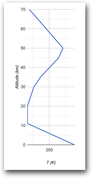
Figure 2. Profile showing temperature versus altitude, US Standard Atmospheric

My calculations for Figure 1 were done from 70 km looking down… but you can see, at that location, the stop in Figure 2 is only 11 km.

So I redid my MODTRAN run shown in Figure 1, this time measuring from the appropriate pauses at each position. You must take two measurements when calculating the longwave change at the breakpoint — one looking up and one looking down. The final answer is the network of two changes.

With that as a prelude, here are my results. I compared them with the results shown in Table 1 by Mhyre et al. paper. My averages are calculated as in Mhyre et al. paper makes the sky clear in the troposphere increases the absorption of long wave (LW) due to double the amount of CO₂ 4.97 watts per square meter (W/m²). This is very close to Mhyre et al. Table 1 figure 5.04 W/m² per double — it’s less than 0.1 W/m² difference. And in addition to the good agreement with the CERES metrics noted in my last post, these results give me confidence in the MODTRAN model.

Figure 3. As shown in Figure 1, the exception is measured at the stop instead of from 70 km to the top of the atmosphere (TOA).

There are a few surprising things about Figure 3. First, there is a slight decrease in the change per doubling as the absolute value of CO in the atmosphere₂ level increased. Surprise. Presumably, this reflects the gradual saturation of the absorption bands. However, it is not large enough to affect most calculations.

Second, and more importantly, I didn’t expect such a big difference between the measurements taken at the two levels. The average TOA measurements are about 52% smaller than the temperature measurements.

This is very interesting as a theory of why an increase in CO2 leads to a warming of the surface. The theory goes like this:

• The amount of CO2 in the atmosphere is increasing.

• This absorbs more of the longer-wave radiation, resulting in peak-atmospheric (TOA) unbalanced radiation. This is the TOA balance between incident sunlight (after some sunlight is reflected back into space) and longwave radiation traveling from the surface and atmosphere.

• To restore balance so that the incoming radiation equals the outgoing radiation, the surface force must heat up until enough additional long waves are present to restore balance.

I pointed out the problem with this theory, that there is some other way to restore TOA balance. Including:

• Increased surface or cloud reflectivity can reduce the amount of sunlight entering.

• Increased absorption of sunlight by aerosols in the atmosphere and clouds can lead to larger swept long waves.

• An increase in the number or duration of thunderstorms moves additional surface heat into the troposphere, moving it above some greenhouse gases and leading to an increase in TOA longwaves.

• An increase in energy from the tropics to the poles increases TOA dài long waves

• A change in the ascending versus descending portion of the atmospheric radiation can lead to an increase in the stratosphere.

Therefore, there is no requirement that the surface temperature increase in response to an increase in CO2. Increasing surface temperature is just one of several ways to restore TOA radiative balance.

With that opening, I understood that the big difference between TOA and troposphere measurement was that I thought the imbalance in TOA was actually due to a doubling of CO₂ will be 3.7 W/m² … But in reality, it’s only about half that, about 1.9 W/m².

Now, as I pointed out above, there are different ways to restore TOA radiation balance. So what percentage of that is from surface warming?

This is the relationship between surface temperature and TOA wavelength.

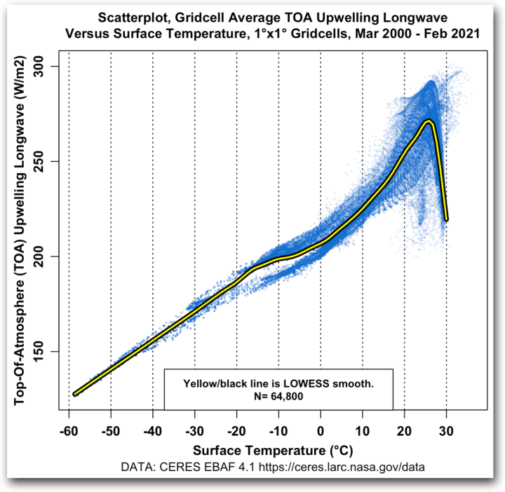
Figure 4. Scatter plot, TOA long wave average elevation above surface temperature, 1° latitude equals 1° grid longitude.

As you might expect, on most of the planet as the surface warms, TOA longwaves increase. This makes sense, a warmer surface radiates more long waves, so you would think TOA longwaves would increase.

But at temperatures above about 26°C, the situation changes rapidly. Above that temperature, the ascending TOA longwave decreases very rapidly as the temperature increases.

I consider this tropical thunderstorm activity. These substances preferentially form at temperatures above ~26°C. Here’s a look at the effect using two very different data sets.

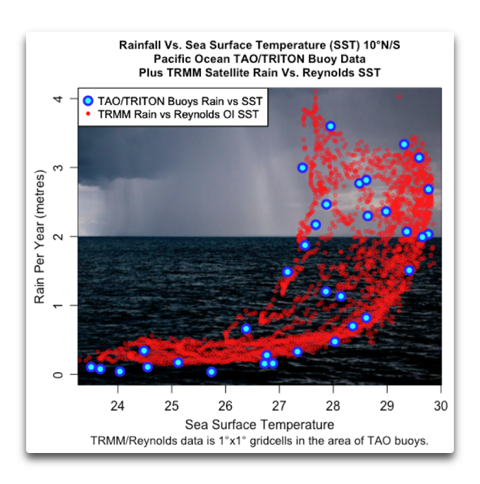
Figure 5. Rainfall from tropical thunderstorms relative to sea surface temperature. The red dots are from the Tropical Rainfall Measurement Mission. The blue dots are from the TAO/TRITON anchor ocean buoy array.

And what is the long-term network of all this across the globe? Figure 6 shows that result.

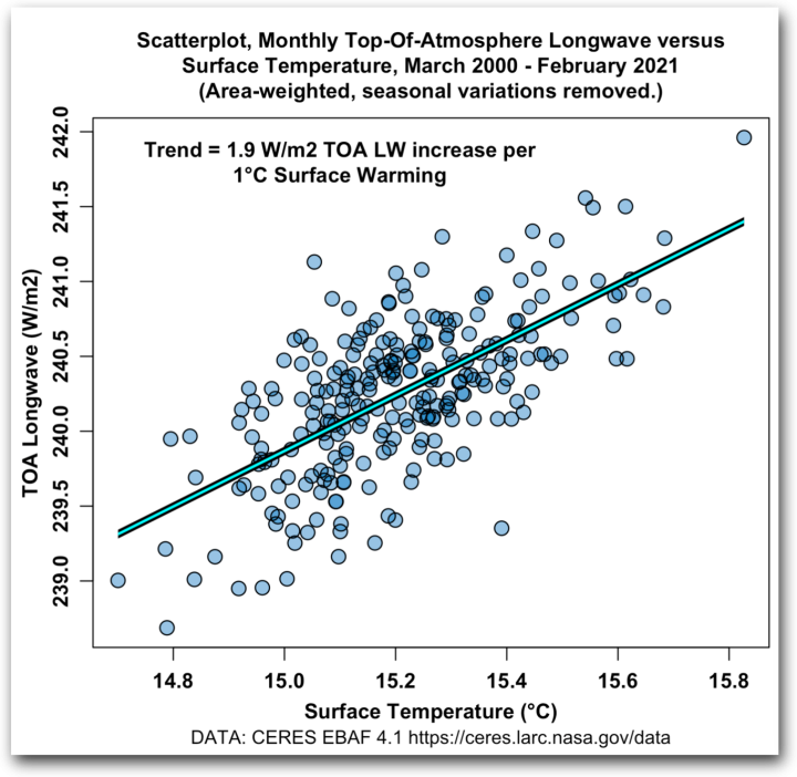
Figure 6. Scatter, monthly high-wavelength pattern of the atmosphere (TOA LW) versus surface temperature.

The other thing is the same (which has never happened), according to CERES data, a 1°C increase in global mean temperature leads to a 1.9 W/m2 increase in TOA LW high-rise housing … which is clearly a Coincidentally, the reduction in TOA LW elevation resulted in a doubling of CO₂.

What’s remarkable in this context is that since we’re dealing with radiation in the atmosphere, everything happens at the speed of light. A cross-correlation analysis showed no delay between the monthly change of surface temperature and the monthly change of TOA longwave.

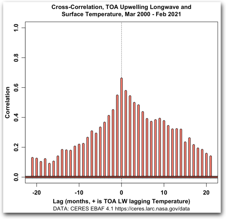
Figure 7. Cross correlation, monthly uppermost atmospheric longwave (TOA LW) and surface temperature. Positive values ​​show the TOA LW hysteresis surface temperature, negative values ​​show the TOA LW hysteresis surface temperature. Overall, there is no lag between the two.

Since there is no hysteresis in this, and since it directly relates surface temperature to the change in TOA longwave radiation, this seems to me to give a good estimate of the gas sensitivity. post-equilibrium (ECS) is 1°C for every doubling of CO₂ … But I know what, I was born yesterday.

Next, the calculated TOA reduction in enhanced LW can account for an increase in HAVE₂ over a 21 year period is about -0.3 W/m². The change in surface temperature over the period was ~0.4°C. This increased TOA LW to ~0.8 W/m² … That is, the surface heats up twice as fast as is required to compensate the TOA imbalance.

Why does the surface heat up faster HAVE₂ increase would suggest? The main reason is an increase in the amount of sunlight absorbed by the surface. That solar added 1.5 W/m² in the 21 year period of the CERES record… as I said, other things never equal.

I extend my best regards to all,

w.

Postscript: In analyzes like this one, it is generally helpful to keep in mind what I humbly call Willis’ “Climate First Rule,” which states

“In the climate, everything is connected to everything else… which in turn is connected to everything else… except that it is not.”

MY USES: I can defend my words, but you cannot interpret mine. When you comment, please REVIEW the EXACT WORDS you are discussing. This avoids endless misunderstandings.