The Effect of a Short Observational Record on the Statistics of Temperature Extremes • Watts Up With That?
New open access paper available in Geophysical Research Letters. H/T Judith Curry
Research Letter Open Access ![]()
The Effect of a Short Observational Record on the Statistics of Temperature Extremes
Joel Zeder, Sebastian Sippel, Olivier C. Pasche, Sebastian Engelke, Erich M. Fischer
First published: 25 August 2023
Abstract
In June 2021, the Pacific Northwest experienced a heatwave that broke all previous records. Estimated return levels based on observations up to the year before the event suggested that reaching such high temperatures is not possible in today’s climate. We here assess the suitability of the prevalent statistical approach by analyzing extreme temperature events in climate model large ensemble and synthetic extreme value data. We demonstrate that the method is subject to biases, as high return levels are generally underestimated and, correspondingly, the return period of low-likelihood heatwave events is overestimated, if the underlying extreme value distribution is derived from a short historical record. These biases have even increased in recent decades due to the emergence of a pronounced climate change signal. Furthermore, if the analysis is triggered by an extreme event, the implicit selection bias affects the likelihood assessment depending on whether the event is included in the modeling.
Key Points
- Standard return period estimates of temperature extremes are systematically overestimated in short records under non-stationary conditions
- The small-sample bias in maximum likelihood estimates is found both for extremes in climate model data and in synthetic data experiments
- Future analysis should account for the statistical implications of the selection bias if the analysis is triggered by an extreme event
Plain Language Summary
In June 2021, the Pacific Northwest experienced a record-breaking heatwave event. Based on historical data, the scientific community has applied statistical models to understand how likely this event was to occur. However, due to the record-shattering nature of this particular heatwave, the model suggested that reaching such high temperatures should not have been possible. In this study, we evaluate the accuracy of these statistical models in describing the occurrence probability of extreme events. We find that the current models tend to underestimate the occurrence probability and that the bias has become more pronounced in recent years due to climate change. Finally, we assess how the way extreme events are included in the model can also affect the accuracy of estimates.
1 Introduction
The heat wave in late June and early July 2021 in the Pacific Northwest (PNW), with temperatures well above previous records, had substantial impacts on mortality, infrastructure, and the ecosystems in the densely populated region (White et al., 2023). This heatwave shattered the long-standing Canadian temperature record by a margin of 4.6°C, and local temperature measurements exceeded previous long-term records by several degrees centigrade even 1 month before temperatures usually peak in this area (Philip et al., 2022). Both the unprecedented event intensity (Thompson et al., 2022) and the severe impacts with several hundred reported excess deaths (Henderson et al., 2022) stimulated exceptional scientific interest in the meteorological drivers (Bartusek et al., 2022; Mo et al., 2022; Neal et al., 2022; Qian et al., 2022; Schumacher et al., 2022; Wang et al., 2023) and the predictability (Emerton et al., 2022; Lin et al., 2022; Oertel et al., 2023).
There is consensus that anthropogenic climate change is the key driver for aggravating hot extremes globally (IPCC, 2021), which also increases the probability of previous temperature records being broken by large margins (Fischer et al., 2021). The extreme event attribution (EEA) study by Philip et al. (2022) concludes that the first-order estimate of the PNW 2021 event frequency is on the order of “once in 1,000 years under current climate conditions,” and that climate change increased the probability by a factor of at least 150. Such statements require estimates of the exceedance probability p1 of the extreme event under current climate conditions, as well as the counterfactual exceedance probability p0 without anthropogenic warming (Allen, 2003; Stott et al., 2016). Estimating the exceedance probability from past observational or reanalysis data is a central step in the EEA protocol (Philip et al., 2020; van Oldenborgh et al., 2021), which usually entails fitting a non-stationary probability distribution whose parameters are a function of global warming. For heatwave attribution studies, the usual choice is fitting a generalized extreme value distribution (GEV) to annual temperature maxima, with the location parameter being linearly dependent on a global mean surface temperature (GMST) covariate. Thereby the full distribution is shifted in line with GMST changes. For annual temperature maxima, the fitted GEV distribution often has an upper bound. This is a consequence of a negative shape parameter, which determines the tail characteristics of the GEV. For the 2021 PNW heatwave, fitting this GEV model to annual temperature maxima prior to the event generally results in an infinite return period estimate, both using gridded reanalysis spatial mean temperature data (Bartusek et al., 2022; Philip et al., 2022) or individual station data (Bercos-Hickey et al., 2022). Figure S1 in Supporting Information S1 shows how the event intensity of 2021 exceeded the estimated upper bound for 2021 by a large margin. By including the event in the GEV fit, Philip et al. (2022) and Bartusek et al. (2022) obtained a finite return period estimate (which is an inherent consequence of the estimation method). Whether or not to include the event is an unresolved question in EEA (Philip et al., 2020), which would require addressing the inherent selection bias, as the analysis is conducted due to the event itself. Also, risk assessment studies are often triggered by record-shattering extreme events that tend to represent outliers, thus they are subject to the same selection bias. The statistical implications of an extreme event trigger on metrics relevant for risk assessment are discussed by Barlow et al. (2020) and Miralles and Davison (2023).
This study aims at assessing the robustness of event probability estimates based on observational data in light of the challenges posed by the PNW 2021 heatwave attribution effort, and which has been observed for several other recent events. To this end, we evaluate the approach by using climate model large ensemble (LE) and synthetic GEV data as a test bed. In Sections 2 and 3, we provide information on the data sets and the statistical procedure used for the evaluation. In Section 4, return level and return period estimates are assessed against the reference values obtained from the pooled ensemble data set, and the implications of the selection bias are discussed.
2 Data
We here use climate model data of an 84 member initial condition LE of the fully coupled Community Earth System Model version 1.2 (CESM1.2; Hurrell et al., 2013) and a 90 member LE of CESM version 2 (CESM2; Danabasoglu et al., 2020). The CESM1.2 ensemble consists of 21 members that cover the historical and future period from 1850 to 2099, of which three additional members each are branched off in 1940. All members follow an RCP8.5 forcing scenario after 2006. The CESM2 ensemble members cover the period from 1850 to 2100 and are forced with an SSP3-7.0 scenario after 2015. The results in the main text are primarily based on CESM1.2 data due to data availability in the initial project phase.
From these models, annual maximum daily average temperature (Tx1d) was retrieved for a domain of 45–50°N, 122.5–120°W (Figure S2 in Supporting Information S1), which is a spatial subset of the domain defined by Philip et al. (2022), but is adjusted to the shared model resolution of 2.5° after interpolation onto a common grid. The GMST covariate, expressed in anomalies against the 1981–2010 average, is obtained from the respective climate models. In accordance with the EEA protocol (Philip et al., 2020), a 4-year running mean low-pass filter is applied to smooth unforced inter-annual variability (Figure S3 in Supporting Information S1). Text S1 in Supporting Information S1 summarizes the respective implementation.
3 Methods
We evaluate 100-year return levels estimated from individual realizations against a reference 100-year return level, which is estimated from the pooled data of all ensemble members or explicitly known in the synthetic data experiments. Given the non-stationarity of the data and the model in Equation 1, the return level estimates are always conditional on the corresponding GMST covariate. Unless further specified, in the following text, “(reference) return level” refers to the 100-year (reference) return level, and “return period” to the estimated return period of the 100-year reference return level.
3.1 Statistical Model
Throughout the study, we model the annual temperature maxima yTx1d as realizations of a non-stationary GEV distribution

(1)
where the location parameter μ is a linear function of the smoothed GMST covariate xGMST
![]()
![]()
![]() (2)
(2)
Following the EEA protocol for heatwave attribution, we here assume a stationary scale parameter σ and shape parameter ξ (Philip et al., 2020; van Oldenborgh et al., 2021). Amplifying processes like land-atmosphere interactions can further increase the variability in heat extremes, thus for example, Bartusek et al. (2022) additionally assume a non-stationary scale parameter.
For a GEV distribution of annual block maxima, the quantile associated with an exceedance probability p is referred to as the return level zp, which would, on average and under stationary conditions, be exceeded every 1/p years. Therefore, the 100-year return level corresponds to the 99% quantile and is shifting with the full distribution as the location parameter changes with GMST, as expressed in Equation 2. We further estimate the return period r = 1/p for a given 100-year reference return level zref,p = 1% as a function of the estimated GEV parameters:
![]()
![]()
![]() (3)
(3)
We put specific focus on estimated return periods, as these directly determine the event probability under current and counterfactual climate conditions and, therefore, attribution metrics like the probability ratio PR = p1/p0 (cf. Section 1).
3.2 Evaluation Steps
We assess return level and return period estimates inferred from individual ensemble members, which are, therefore, only subject to (random) sampling uncertainty and differences due to internal climate variability. In the first step, we estimate the reference values from a non-stationary reference GEV model, which is fitted to the entire ensemble data set (pooling all members in a LE), against which the estimates from individual ensemble members are assessed. Text S2 in Supporting Information S1 summarizes the evaluation of the reference return level estimates concerning the questions of (a) whether a block size of 1 year yields stable results and (b) whether the model formulation in Equation 1 sufficiently captures the complexity in the data. In short, the reference return level values of the base model in Equation 1 are found to be consistent with such derived from more complex extreme value models and for larger block sizes.
In a next step, for each individual ensemble member, a GEV model is fitted to either the complete available Tx1d time series (i.e., 1850–2099, referred to as long estimation period), but also to 71-year sub-periods (e.g., 1950–2020, referred to as short estimation period), as shown in Figure 1a. The former is only used to infer the effect on GEV parameter estimates when all historical and future data are available (the impact on the trend parameter μGMST is shown in Figure 1b). The return level and return period estimates are then evaluated against the reference values at the smooth ensemble-mean GMST level of the year following the estimation period (e.g., 2021, see Figure 1c).
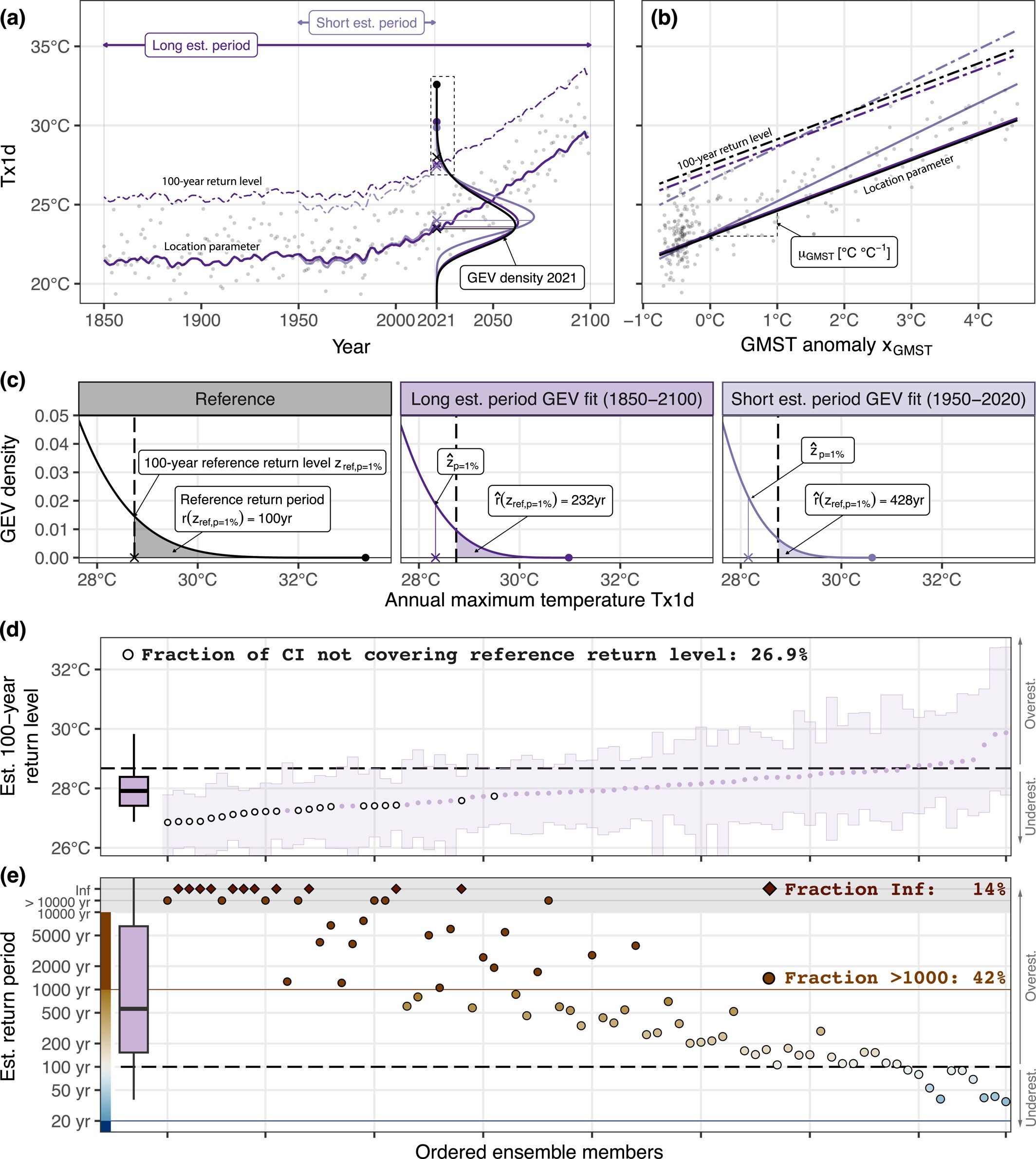
 as shaded area. (d) Ordered maximum likelihood 100-year return level estimates (dots) and non-parametric bootstrap confidence intervals (CI) (shaded area, filled white dots highlight estimates where the CI does not cover the reference return level), and (e) corresponding return period estimates. Box plots summarize the respective distributions (box: 25%–75%, whiskers: 1%–99%). Corresponding Bayesian estimates and long estimation period results, and CESM2 results and are shown in Figures S4 and S5 of the Supporting Information S1.
To assess the effect of the estimation procedure, parameters were estimated with classical maximum likelihood (ML) but also with Bayesian posterior sampling. An excellent introduction to non-stationary extreme value modeling covering both estimation approaches is provided by Coles (2001). For the former, 95% confidence intervals (CI) are retrieved using non-parametric bootstrapping, the default approach suggested in the EEA protocol (Philip et al., 2020). Bayesian point estimates are calculated as posterior means, and central credible intervals (also abbreviated CI), that is, 2.5%–97.5% quantiles of the posterior distribution, are obtained as uncertainty measures for the Bayesian estimates. Text S1 in Supporting Information S1 provides further background on the technical implementation of the estimation procedure.
Additionally, evaluations are conducted in synthetic data experiments, where samples are drawn from a pre-defined GEV distribution as in Equation 1. From these, estimates are obtained by re-fitting the same GEV model, providing an independent data set to assess return level and return period estimates, but for data that follows the assumed GEV model by design. The “static” synthetic data experiment resembles the PNW 2021 attribution study (with a fixed estimation period 1950–2020), with varying GEV reference parameters and GMST covariate time series (resembling the LE setup). Furthermore, two additional synthetic data experiments are conducted to evaluate the quality of ML estimates over time (“transient” experiment) and for increasingly large estimation data sets (“sample size experiment”). Detailed methods and results are provided in Text S3 of the Supporting Information S1 and are referenced throughout the following results section.
4 Results and Discussion
Based on LE climate model data, we first demonstrate a systematic underestimation of the return level and a corresponding overestimation of the return period for an estimation period 1950–2020, analogous to the PNW 2021 attribution study. Later, we expand the analysis to further estimation periods to explore the temporal evolution of the bias. We also outline the effect of a potential selection bias and the consequences of including or not including the extreme or record-breaking event when estimating its return level.
4.1 Systematically Underestimated Return Levels of Temperature Extremes
The right panel in Figure 1c illustrates a GEV model fitted with ML to data of an individual climate model ensemble member for the short estimation period 1950–2020, in which the corresponding return level is lower than the reference return level calculated from all members. Therefore, the estimated return period is much higher than what it should be, that is, 100 years. While this specific ensemble member shown in Figures 1a–1c is just one illustrative case, a key result of our study is that the majority of estimated 100-year return levels fall below the reference return level. This can be seen in Figure 1d, where return levels estimated from individual ensemble members are shown in ascending order along with their actual reference return level (horizontal dashed line, the box plot on the left summarizes the distribution of estimates). Our results show a negative bias in ML estimates of high return levels due to the short estimation period. In principle, for individual members, this result could also arise due to random sampling uncertainty, but the reference value should then fall within the respective CI at the rate of the corresponding confidence level. The CI in Figure 1d, however, show that the fraction of CI not including the reference value amounts to 26.9%, a ratio much larger than the 5% expected for 95% CI, which is referred to as under-coverage. Furthermore, if not covered by the CI, the reference value should fall evenly above and below the CI, which is not the case. Bayesian CI, on the other hand, tend to have too high coverage (Figure S5a in Supporting Information S1), as for all the estimates, the respective 95% CI cover the reference return level.
The systematic underestimation of 100-year return levels in relatively short temperature records implies an underestimation of the exceedance probability of the 100-year reference return level, that is, an overestimation of the return period, as visualized in the right panel of Figure 1c. Figure 1e shows a clear correspondence between return period and the respective 100-year return level estimates (Figure 1d). In 41% of the cases, the return period of an event with a “true” return period of 100 years is estimated to be larger than 1,000 years. In 14% of ensemble members, a 100-year event is even considered to have zero exceedance probability or infinite return period. These results indicate a substantial risk of overestimating the return period when the record of observations used for the statistical analysis is limited. This result has serious implications for adaptation and planning. Temperatures that are estimated to be never reached may actually be exceeded with a 1% probability in a given year (i.e., have a 100-year return period). The large sensitivity of return period estimates is a consequence of the bounded short-tail nature of heat extremes, such that return periods can be overestimated by orders of magnitude if not reaching infinity. In the following sections, we further discuss how this bias evolves for different estimation periods and methods.
4.2 Temporary Bias Amplification
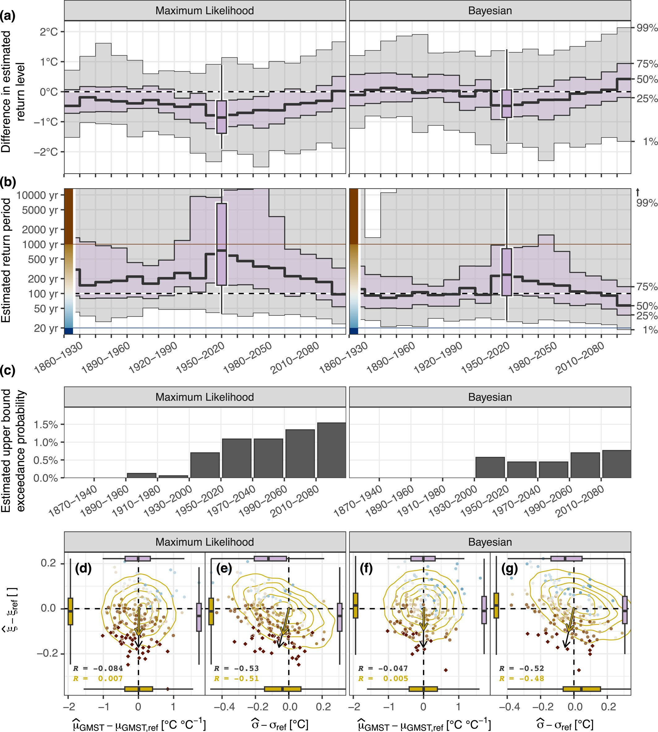
The previous paragraphs outline the underestimation of return levels and the overestimation of return periods for GEV fits in individual ensemble members and the estimation period 1950–2020, evaluated in 2021. In the following, we investigate whether the underestimation of the return level is also influenced by the fact that 2021 falls in a period of rapid warming. Figure 2 shows the distribution of return level (Figure 2a) and return period (Figure 2b) estimates for overlapping 71-year estimation periods (1850–1920, 1851–1921, etc.), aggregated per decade (shaded background), and explicitly for the 1950–2020 estimation period (box plot). We find a roughly constant underestimation in return levels and an overestimation in return periods for estimation periods ending before 1990. For periods ending after 1990, the biases substantially increase temporarily and diminish again toward the end of the century. We further observe a strong increase in the fraction of events whose intensity exceeds the estimated upper bound of the GEV distribution derived from the preceding 71-year estimation period, analogous to the PNW 2021 event (Figure 2c; Text S4 in Supporting Information S1).
 (y-axis), and the trend parameter
  and scale parameter
  (x-axis) relative to their reference value (combined 1950–2020 CESM1.2 and CESM2 estimates are shown). The color of the points refers to the corresponding return period value (as in diamonds mark infinite return periods), the arrows show the direction of the respective gradient. Yellow density contour lines illustrate the distribution of estimates in the “static” synthetic data experiment, with the corresponding yellow gradient vector. Box plots on the side summarize the respective marginal distributions (magenta for the large ensemble data points, yellow for the synthetic data), and the Pearson correlation value R is provided in the bottom left corner.
The time dependence and especially the steep increase of return level and return period biases for periods ending after 1990 are likely to be caused by the fact that a majority of Tx1d data used for the model fit are close to stationary with a weak warming trend. In a period of rapid accelerating warming, non-stationarity and further climate and statistical issues may affect the statistical model and associated biases: Nonetheless, an analysis of the estimated GEV parameters reveals that the temporary overestimation of return periods cannot be attributed to an underestimation of the trend parameter 
; first, the estimates are largely unbiased with respect to the reference value (horizontal magenta box plot in Figures 2d and 2f), and second, the effect of  on the estimated return period is negligible, when compared to the effect of an under- or overestimation of the shape parameter
  (the return period increases almost exclusively along the y-axis with decreasing values of
  , visualized by the black gradient arrow in Figures 2d and 2f). In contrast, the scale parameter
  is subject to a negative bias (horizontal magenta box plot in Figures 2e and 2g) and an underestimation of
  promotes overestimating the return period (tilted gradient arrow in Figures 2e and 2g), but an underestimation of
  is often compensated by an overestimation of
  (and vice versa, the correlation being R ≈ −0.5). The attribution of the temporary return period overestimation bias to specific GEV parameters is therefore not straightforward, but we conclude that a necessary condition is an underestimation of the shape parameter
  . The distribution of estimates from the “static” synthetic data experiment (yellow contours) confirms the relationship between estimates (similar correlation values) and the relative effect strength of individual parameters on return period estimates (yellow gradient arrows) found in LE-based estimates.
A temporary return period bias is also not present in synthetic GEV data generated in the “transient” experiment with a non-stationary forced response GMST covariate (Text S3.3 in Supporting Information S1), where the biases are found to be constant over time (Figure S7 in Supporting Information S1). This discrepancy between climate model and synthetic GEV data has two potential explanations; the statistical model is less capable of successfully detecting and accounting for the non-stationarity since the Tx1d data from LE data is not perfectly GEV-distributed. Alternatively, the temporal variation in the biases might be due to model misspecification, as additional forcing agents (modes of internal variability, local effects of volcanic and anthropogenic aerosols, as considered by Risser et al. (2022)) are not accounted for in the GMST-dependent GEV model formulation in Equation 2. Such additional forcing agents could be accounted for by including further covariates, however, this approach comes at the cost of lower regional generalizability (if very specific forcing agents are considered for the respective location) and higher model complexity (more parameters have to be estimated).
In summary, the GEV model correctly identifies the positive trend in Tx1d intensity also in today’s climate with a high warming rate after a period of weaker warming before 1990. Nonetheless, the temporary overestimation of return periods indicates an increased sensitivity to discrepancies between physical climate variables and statistical model specifications. This has implications both for risk assessment and EEA. The underestimation of return levels and the under-coverage of the respective CI can result in an underestimation of the risk associated with extreme heatwave events. The tendency to overestimate the return period of observed extreme heatwave events may fuel the impression that seemingly impossible heatwave extremes are currently clustering at an unprecedented rate.
4.3 Sensitivity to Methodological Choices
In the following, we briefly evaluate whether the bias in return level and return period estimates is sensitive to the underlying estimation method. Comparing the offsets in return level and return period estimates, Figure 2 suggests smaller biases in Bayesian (right panels) compared to ML estimates (left panels). The agreement in ML and Bayesian GEV parameter estimates across ensemble members is extremely high (with correlations above 0.96 for all parameters, as shown in the diagonal panels of Figure S8 in Supporting Information S1), thus there are no fundamental differences between ML and Bayesian model fits. However, Bayesian scale and shape parameters are estimated slightly higher, which partly explains the smaller bias in return level and return period estimates (Figures 2f and 2g).
This investigation is complemented by two synthetic GEV data experiments, where the data follows a GEV distribution by construction. In the “static” synthetic data experiment (Text S3.1 in Supporting Information S1), where ML and Bayesian estimates are directly compared, we also find that ML return period estimates are subject to a systematic offset; 50% of ML return period estimates for the reference 100-year return level are larger than 200 years (Figure S9a in Supporting Information S1). Thus, the biases found in climate model data are clearly not only due to the data not truly following a GEV distribution, but are even found when the underlying data is GEV distributed by construction. Bayesian return period estimates, on the other hand, are largely unbiased, but still, return period estimates of infinity may be reached in a few individual cases. The underlying Bayesian scale and shape parameter estimates are again slightly higher than the corresponding ML estimates (Figures 2f and 2g; Figure S10 in Supporting Information S1), which leads to the alleviated mean bias, and thus confirms the pattern found in estimates derived from climate model data (Figure S8 in Supporting Information S1). Roodman (2018) and Bücher and Zhou (2021) discuss the sub-asymptotic “small-sample” bias of ML derived GEV parameter and return level estimates, which we further investigate in a second “increasing sample size” synthetic data experiment (Text S3.2 in Supporting Information S1). The “small-sample” bias primarily affects the shape parameter, and its direction also depends on the value of the latter, that is, a negative shape is systematically underestimated, and vice versa. This bias propagates and consequently also affects return level and return period estimates (Figure S11 in Supporting Information S1).
4.4 The Implications of the Selection Bias
In the following, we here briefly discuss the implications of the implicit stopping rule, that is, the fact that many scientific papers or risk evaluations are motivated by a very extreme event in observations or model data that needs to be put into context. In such a study, it is often unclear whether or not the respective event should then be used for the fit. This question is particularly relevant for record-breaking or record-shattering events at the end of the observational record, that is, events that are addressed in EEA studies and often initiate a reevaluation of previously estimated climate risk. The GEV analysis assumes that the extreme event in question is an independent and identically distributed sample of the same distributions as the previous observations. However, as the analysis was triggered by the extremeness of the event to be evaluated (a so-called stopping rule is applied), both including or excluding the event will induce a bias (Barlow et al., 2020).
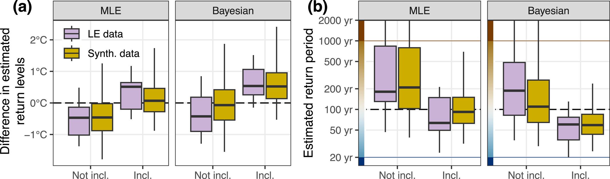
We analyze the effect of including or not including the event of interest at the end of the records by assessing how it affects return level and return period estimates. To this end, we search for events in the LE data sets that have a “true” return period of at least 100 years (based on the reference GEV model). Then we compare the estimated return level and return period estimated from two 71-year estimation periods, where one does and the other does not include the event in question (e.g., for an extreme event in 2051, we compare estimates of the two periods 1980–2050 and 1981–2051). Adding 1 year with a very extreme event strongly changes the GEV fit, as Figure 3 confirms the expectation that including the event results in an overestimation of the return level and an underestimation of the return period. This reversal in the sign of the biases has the interesting effect, that the relative biases in Bayesian estimates are now larger than in ML estimates. This means that Bayesian estimates are not more accurate in both scenarios, and should thus not be considered superior per se. Corresponding estimates from synthetic data of a stationary GEV reveal a similar pattern, but biases are generally smaller.
Barlow et al. (2020) discuss the consequences of the stopping rule in extreme event analysis and propose an adjustment of the likelihood function. With minor adjustments and few considerations regarding the triggering threshold, the method of Barlow et al. (2020) could allow for a more stringent handling of the implicit stopping rule in EEA and risk assessment, as demonstrated by Miralles and Davison (2023) for the PNW 2021 heatwave attribution.
5 Conclusions and Outlook
In this study, we assess different challenges in accurately estimating high return levels and the return period of extreme heatwave events on the basis of short observational records. This evaluation is motivated by the record-shattering PNW 2021 heatwave, where the respective extreme value model derived from observations up to the year before the event suggested an infinite return period or zero probability of reaching the observed event intensity. This raised the question of whether the non-stationary statistical approach widely used in risk assessments, adaptation planning, or EEA, is reliable.
We find that heatwave return levels estimated from limited records are systematically underestimated, which is further aggravated by the fact that the associated CI also underestimate the associated uncertainty range. This bias can result in an underestimation of the associated heatwave risk, which is relevant for adaptation and infrastructure planning. It further translates into an overestimation of the return period of observed extreme events, especially under the strong warming conditions of recent decades. Even though LE climate model data provide a robust test bed, we further verified the evaluation results in targeted synthetic data experiments in which the data is GEV distributed by construction. We identify the ML sub-asymptotic “small-sample” bias in GEV parameter and return level estimates, which only vanishes for sample sizes unattainable in the context of current observational heatwave records.
The offset in Bayesian return level and return period estimates is substantially smaller if the triggering extreme event is not included. Aside from more fundamental considerations (Mann et al., 2017; Shepherd, 2021; Stott et al., 2017), certain practical advantages would call for Bayesian extreme value modeling; more transparency regarding model choices (e.g., priors used for the shape parameter), or the ability to use a joint statistical modeling framework for observational and climate model data (Ribes et al., 2020; Robin & Ribes, 2020) and to avoid artifacts caused by the boundedness of the GEV distribution (Castro-Camilo et al., 2022). We also strongly advocate thoroughly considering the selection bias whenever future analyses are triggered by an extreme event, for example, through implementing the measures suggested by Barlow et al. (2020) and Miralles and Davison (2023). Furthermore, alternative ML-based approaches to derive CI for GEV parameters and return levels should be considered; for example, profile likelihood CI could help to reduce the under-coverage found for return level CI (Coles, 2001).
In summary, our results show that the systematic overestimation of the return periods is largest for short observational periods, in today’s climate when a rapidly warming period follows a period of less or no warming, and for studies focusing on record-breaking and record-shattering temperature extremes. Thereby it affects many recent studies and reports, and it is crucial that those biases are taken into account when putting such events into a climate context, in all fields from adaptation and planning to communication of event attribution.
Acknowledgments
J.Z. and E.M.F. acknowledge funding from the Swiss National Science Foundation within the project “Understanding and quantifying the occurrence of very rare climate extremes in a changing climate” (Grant 200020_178778). S.S. and E.M.F. acknowledge funding from the European Union H2020 project “Extreme events: Artificial intelligence for detection and attribution” (XAIDA; Grant 101003469). O.P. and S.E. acknowledge funding from the Swiss National Science Foundation Eccellenza Grant “Graph structures, sparsity and high-dimensional inference for extremes” (Grant PCEGP2_186858). We thank C. Barnes and F. Otto for the extensive discussion of the results and their constructive and detailed feedback on the model evaluation. We further thank A. Ferreira and L. Belzile for their statistical input on the small-sample bias. The analysis was carried out in R (R Core Team, 2022), thus we thank all contributors for the numerous R packages crucial for this work.
Data Availability Statement
Pre-processed large ensemble data and estimated GEV data are available at https://doi.org/10.3929/ethz-b-000619286. R code (R Core Team, 2022) for pre-processing of data, GEV model estimation from large ensemble data, evaluation of return level and return period estimates, and simulation experiments is available on https://doi.org/10.5281/zenodo.8118283. All original ERA5 reanalysis data (Hersbach et al., 2020) used in this study are publicly available on https://doi.org/10.24381/cds.adbb2d47.
Supporting Information
Please note: The publisher is not responsible for the content or functionality of any supporting information supplied by the authors. Any queries (other than missing content) should be directed to the corresponding author for the article.
References
- Allen, M. (2003). Liability for climate change. Nature, 421(6926), 891–892. https://doi.org/10.1038/421891a
- Barlow, A. M., Sherlock, C., & Tawn, J. (2020). Inference for extreme values under threshold-based stopping rules. Journal of the Royal Statistical Society Series C: Applied Statistics, 69(4), 765–789. https://doi.org/10.1111/rssc.12420
- Bartusek, S., Kornhuber, K., & Ting, M. (2022). 2021 North American heatwave amplified by climate change-driven nonlinear interactions. Nature Climate Change, 12(12), 1143–1150. https://doi.org/10.1038/s41558-022-01520-4
- Bercos-Hickey, E., O’Brien, T. A., Wehner, M. F., Zhang, L., Patricola, C. M., Huang, H., & Risser, M. D. (2022). Anthropogenic contributions to the 2021 Pacific Northwest heatwave. Geophysical Research Letters, 49(23), 1–17. https://doi.org/10.1029/2022GL099396
- Bücher, A., & Zhou, C. (2021). A horse race between the block maxima method and the peak–over–threshold approach. Statistical Science, 36(3), 360–378. https://doi.org/10.1214/20-STS795
- Castro-Camilo, D., Huser, R., & Rue, H. (2022). Practical strategies for generalized extreme value-based regression models for extremes. Environmetrics, 33(6), 1–14. https://doi.org/10.1002/env.2742
- Coles, S. (2001). An introduction to statistical modeling of extreme values ( 3rd print ed.). Springer.
- Danabasoglu, G., Lamarque, J., Bacmeister, J., Bailey, D. A., DuVivier, A. K., Edwards, J., et al. (2020). The community Earth system model version 2 (CESM2). Journal of Advances in Modeling Earth Systems, 12(2), 1–35. https://doi.org/10.1029/2019MS001916
- Emerton, R., Brimicombe, C., Magnusson, L., Roberts, C., Di Napoli, C., Cloke, H. L., & Pappenberger, F. (2022). Predicting the unprecedented: Forecasting the June 2021 Pacific Northwest heatwave. Weather, 77(8), 272–279. https://doi.org/10.1002/wea.4257
- Fischer, E. M., Sippel, S., & Knutti, R. (2021). Increasing probability of record-shattering climate extremes. Nature Climate Change, 11(8), 689–695. https://doi.org/10.1038/s41558-021-01092-9
- Henderson, S. B., McLean, K. E., Lee, M. J., & Kosatsky, T. (2022). Analysis of community deaths during the catastrophic 2021 heat dome. Environmental Epidemiology, 6(1), e189. https://doi.org/10.1097/EE9.0000000000000189
- Hersbach, H., Bell, B., Berrisford, P., Hirahara, S., Horányi, A., Muñoz-Sabater, J., et al. (2020). The ERA5 global reanalysis. Quarterly Journal of the Royal Meteorological Society, 146(730), 1999–2049. https://doi.org/10.1002/qj.3803
- Hurrell, J. W., Holland, M. M., Gent, P. R., Ghan, S., Kay, J. E., Kushner, P. J., et al. (2013). The community Earth system model: A framework for collaborative research. Bulletin of the American Meteorological Society, 94(9), 1339–1360. https://doi.org/10.1175/BAMS-D-12-00121.1
- IPCC. (2021). Summary for policymakers. In V. Masson-Delmotte, R. Allan, P. Arias, S. Berger, J. G. Canadell, C. Cassou, D. Chen, et al. (Eds.), Climate change 2021: The physical science basis. Contribution of working group I to the sixth assessment report of the intergovernmental panel on climate change (pp. 3–32). Cambridge University Press. https://doi.org/10.1017/9781009157896.001
- Lin, H., Mo, R., & Vitart, F. (2022). The 2021 western North American heatwave and its subseasonal predictions. Geophysical Research Letters, 49(6), 1–10. https://doi.org/10.1029/2021GL097036
- Mann, M. E., Lloyd, E. A., & Oreskes, N. (2017). Assessing climate change impacts on extreme weather events: The case for an alternative (Bayesian) approach. Climatic Change, 144(2), 131–142. https://doi.org/10.1007/s10584-017-2048-3
- Miralles, O., & Davison, A. C. (2023). Timing and spatial selection bias in rapid extreme event attribution. Weather and Climate Extremes, 41, 100584. https://doi.org/10.1016/j.wace.2023.100584
- Mo, R., Lin, H., & Vitart, F. (2022). An anomalous warm-season trans-Pacific atmospheric river linked to the 2021 western North America heatwave. Communications Earth & Environment, 3(1), 127. https://doi.org/10.1038/s43247-022-00459-w
- Neal, E., Huang, C. S. Y., & Nakamura, N. (2022). The 2021 Pacific Northwest heat wave and associated blocking: Meteorology and the role of an upstream cyclone as a diabatic source of wave activity. Geophysical Research Letters, 49(8), e2021GL097699. https://doi.org/10.1029/2021GL097699
- Oertel, A., Pickl, M., Quinting, J. F., Hauser, S., Wandel, J., Magnusson, L., et al. (2023). Everything hits at once: How remote rainfall matters for the prediction of the 2021 North American heat wave. Geophysical Research Letters, 50(3), e2022GL100958. https://doi.org/10.1029/2022GL100958
- Philip, S. Y., Kew, S., van Oldenborgh, G. J., Anslow, F. S., Seneviratne, S. I., Vautard, R., et al. (2022). Rapid attribution analysis of the extraordinary heat wave on the Pacific coast of the US and Canada in June 2021. Earth System Dynamics, 13(4), 1689–1713. https://doi.org/10.5194/esd-13-1689-2022
- Philip, S. Y., Kew, S., van Oldenborgh, G. J., Otto, F., Vautard, R., van der Wiel, K., et al. (2020). A protocol for probabilistic extreme event attribution analyses. Advances in Statistical Climatology, Meteorology and Oceanography, 6(2), 177–203. https://doi.org/10.5194/ascmo-6-177-2020
- Qian, Y., Hsu, P., Yuan, J., Zhu, Z., Wang, H., & Duan, M. (2022). Effects of subseasonal variation in the East Asian monsoon system on the summertime heat wave in western North America in 2021. Geophysical Research Letters, 49(8), e2021GL097659. https://doi.org/10.1029/2021GL097659
- R Core Team. (2022). R: A language and environment for statistical computing. R Foundation for Statistical Computing. Retrieved from https://www.r-project.org/
- Ribes, A., Thao, S., & Cattiaux, J. (2020). Describing the relationship between a weather event and climate change: A new statistical approach. Journal of Climate, 33(15), 6297–6314. https://doi.org/10.1175/JCLI-D-19-0217.1
- Risser, M. D., Collins, W. D., Wehner, M. F., O’Brien, T. A., Paciorek, C. J., O’Brien, J. P., et al. (2022). A framework for detection and attribution of regional precipitation change: Application to the United States historical record. Climate Dynamics, 60(3–4), 705–741. https://doi.org/10.1007/s00382-022-06321-1
- Robin, Y., & Ribes, A. (2020). Nonstationary extreme value analysis for event attribution combining climate models and observations. Advances in Statistical Climatology, Meteorology and Oceanography, 6(2), 205–221. https://doi.org/10.5194/ascmo-6-205-2020
- Roodman, D. (2018). Bias and size corrections in extreme value modeling. Communications in Statistics—Theory and Methods, 47(14), 3377–3391. https://doi.org/10.1080/03610926.2017.1353630
- Schumacher, D. L., Hauser, M., & Seneviratne, S. I. (2022). Drivers and mechanisms of the 2021 Pacific Northwest heatwave. Earth’s Future, 10(12), 9156. https://doi.org/10.1029/2022EF002967
- Shepherd, T. G. (2021). Bringing physical reasoning into statistical practice in climate-change science. Climatic Change, 169(1–2), 1–19. https://doi.org/10.1007/s10584-021-03226-6
- Stott, P. A., Christidis, N., Otto, F. E. L., Sun, Y., Vanderlinden, J., van Oldenborgh, G. J., et al. (2016). Attribution of extreme weather and climate-related events. WIREs Climate Change, 7(1), 23–41. https://doi.org/10.1002/wcc.380
- Stott, P. A., Karoly, D. J., & Zwiers, F. W. (2017). Is the choice of statistical paradigm critical in extreme event attribution studies? Climatic Change, 144(2), 143–150. https://doi.org/10.1007/s10584-017-2049-2
- Thompson, V., Kennedy-Asser, A. T., Vosper, E., Lo, Y. T. E., Huntingford, C., Andrews, O., et al. (2022). The 2021 western North America heat wave among the most extreme events ever recorded globally. Science Advances, 8(18), 1–11. https://doi.org/10.1126/sciadv.abm6860
- van Oldenborgh, G. J., van der Wiel, K., Kew, S., Philip, S., Otto, F., Vautard, R., et al. (2021). Pathways and pitfalls in extreme event attribution. Climatic Change, 166(1–2), 13. https://doi.org/10.1007/s10584-021-03071-7
- Wang, C., Zheng, J., Lin, W., & Wang, Y. (2023). Unprecedented heatwave in western North America during late June of 2021: Roles of atmospheric circulation and global warming. Advances in Atmospheric Sciences, 40(1), 14–28. https://doi.org/10.1007/s00376-022-2078-2
- White, R. H., Anderson, S., Booth, J. F., Braich, G., Draeger, C., Fei, C., et al. (2023). The unprecedented Pacific Northwest heatwave of June 2021. Nature Communications, 14(1), 727. https://doi.org/10.1038/s41467-023-36289-3
References From the Supporting Information
- Ciavarella, A., Cotterill, D., Stott, P., Kew, S., Philip, S., van Oldenborgh, G. J., et al. (2021). Prolonged Siberian heat of 2020 almost impossible without human influence. Climatic Change, 166(1–2), 9. https://doi.org/10.1007/s10584-021-03052-w
- Hansen, J., Ruedy, R., Sato, M., & Lo, K. (2010). Global surface temperature change. Reviews of Geophysics, 48(4), 1–29. https://doi.org/10.1029/2010RG000345
- Vautard, R., van Aalst, M., Boucher, O., Drouin, A., Haustein, K., Kreienkamp, F., et al. (2020). Human contribution to the record-breaking June and July 2019 heat waves in western Europe. Environmental Research Letters, 15(9), 094077. https://doi.org/10.1088/1748-9326/aba3d4
- Youngman, B. D. (2022). Evgam: An R package for generalized additive extreme value models. Journal of Statistical Software, 103(3). https://doi.org/10.18637/jss.v103.i03