Guest Post by Willis Eschenbach
This is the third post looking at the use of grid-based scatter plots of 1° longitude by 1° latitude. First lesson, Global Dispersion, considered a grid-based scatter plot of surface cloud radiation (CRE) effects versus temperature. CRE measures how well clouds warm or cool the surface through a combination of their effects on shortwave (solar) and longwave (heat) radiation.
Figure 1. Original caption: Scatter plot, surface temperature (horizontal “x” axis) versus radiation effect of real surface cloud (vertical “y” axis). Gives a new meaning to the word “non-linear”.
The slope of the yellow/black line shows the change in CRE for each 1°C change in temperature. Note the rapid amplification of the cooling cloud above about 25°C.
Second post, Sun sensitivityused the same method to investigate the relationship between available solar energy (top of the atmosphere [TOA] sun minus albedo reflectance) and temperature. Here is the image from that post.
Figure 2. Original caption: Scatterplot, cellcell-by-gridcell surface temperature relative to available solar energy. Number of grid cells = 64,800. The cyan/black line represents the LOWEST smoothness of the data. The slope of the cyan/black line shows the temperature change for each 1 W/m2 change in available solar energy. The data in all of these posts is an average of all 21 years of CERES data.
As before, the slope of the cyan/black line shows the change in surface temperature per W/m2 change in available solar energy.
In this section, the point of interest is the three roughly aligned sections, especially the right one. In that section, the additional solar does not raise the temperature.
Figure 3 below shows the slope of the cyan/black line relative to available solar energy.
Figure 3. Original caption: The slope of the trend line in Figure 2. This shows the amount of temperature change for a 1 W/m2 change in available solar energy.
This method of looking at data is of great interest because it shows long-term relationships between variables. Each grid cell has had thousands of years to balance with its overall current temperature and available solar energy. So looking at the temperatures of both near and far grid cells with slightly different solar availability reveals a long-term relationship between solar energy and temperature, not what happens. with rapid change.
Next, it is valuable because the slope is relatively insensitive to changes in mean temperature or available average solar energy. Changes in mean temperature only move the cyan/black line up or down, but this causes very little change in slope on the cyan/black line.
Similarly, changes in average solar move the cyan/black line left or right. And changes in both mean temperature and mean solar shift the data diagonally…but none of this changes the variable of interest, the slope of the cyan/black line, according to in any significant way.
Now, for this post, I want to look at the relationship between the very poorly named “greenhouse” radiation and surface temperature.
And what is greenhouse radiation when it’s at home?
All solid objects, including the earth, emit thermal radiation. That’s how night vision goggles work. They allow us to “see” that radiation.
Some radiation from the earth goes straight out into space. But some is absorbed by the atmosphere. This is eventually re-projected in all directions, with about half going up and half facing back to earth. This long-wave thermal radiation that travels down (towards the earth) is called “greenhouse radiation”.
Now, a smart guy named Ramanathan has shown that we can actually measure this amount of greenhouse radiation from space. For each grid cell, we take the amount of radiation emitted on the surface. From that, we subtract the radiation escaping into space. The rest is what has been absorbed by the atmosphere and directed downwards – greenhouse radiation.
So I wanted to see what happens to the surface temperature when the greenhouse irradiance changes. But there is an immediate problem. The amount of greenhouse radiation increases and decreases whenever the surface temperature changes. If the surface is warmer and more radiating, more will be absorbed by the atmosphere, and as the surface temperature increases, more greenhouse radiation will be emitted.
To remove that difficulty, we can express the greenhouse effect as a percentage of the long-wave surface radiation (directed into space). This eliminates the direct influence of surface temperature on greenhouse radiation. Figure 4 shows the resulting relationship between surface temperature and greenhouse effect as a percentage of laminar irradiance.
Figure 4. Scatterplot, plot surface temperature as a percentage of greenhouse irradiance. Number of grid cells = 64,800. The red/black line shows the LOWEST smoothness of the data. The slope of the cyan/black line shows the temperature change for each 1 W/m2 change in available solar energy. A few negative grid cells are located at the poles, and they show the effect of heat input from the tropics.
And here is the corresponding graph of the slope, when the percentage is converted back to W/m2.
Figure 5. Slope of the trend line in Figure 4. This shows the amount of change in temperature for a 1 W/m2 change in greenhouse irradiance.
This has both similarities and differences from the warming caused by changes in solar energy availability shown in Figure 3 above. Both start high on the left, and both end with an unchanged low slope on the right. However, the warming of the greenhouse in the middle is much greater. This results in a global region-average climate sensitivity of 0.58°C per 1 W/m2 of additional greenhouse irradiance.
This equates to about 2°C for each CO2 doubling. This is about the same level of equilibrium climate sensitivity found by Nic Lewis in his recent study Objectively incorporate climate-sensitive evidenceviz:
Estimates of long-term climate sensitivity are much lower and more constrained (average 2.16 °C, 17–83% between 1.75–2.7 °C, 5–95 % in the range of 1.55–3.2 °C) compared to Sherwood et al. and at AR6 (central value 3°C, most likely between 2.0–5.0°C).
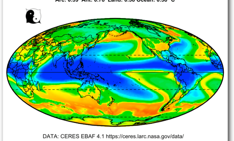
Finally, this method gives an estimate of the climate sensitivity for each grid cell. Here’s that map, showing how much the estimated surface temperature changes for each additional W/m2 of greenhouse radiation.
Figure 6. Expected temperature change due to greenhouse radiation increase of 1 W/m2.
This makes sense. The areas in blue are the locations of the Intertropical Convergence and the Western Pacific Warm Water Basin. They are usually covered by cumulus and thunderstorm clouds. These act as a 100% absorber of high-level radiation… so any additional CO2 will make little difference. Also, the temperatures in these areas are close to the maximum, so they won’t warm up much due to increased solar radiation or greenhouses.
Well, there are probably more insights to be drawn from all of this. But this post is long enough, so I’ll leave it at that. For example, I’m sure I can get better results by breaking down the data, by both northern/southern hemisphere and land vs ocean. That would do better than just comparing like with like. But sadly, there are never enough hours, in a day or a lifetime
And as usual, what I found raised more questions than answers. I treat my writings in a sense as a constant notebook in my lab where I can have a permanent record of what I’m finding and you can learn. about things when and when I learn about them.
Best wishes to all of you, and thank you for your continued interest, participation, and critique of my ongoing investigations into the mysteries of this amazing universe,
w.
My perennial request: When you comment, please quote exactly the words you are discussing. It avoids all kinds of misunderstandings.
Previous job: There is an index for my work here, divided by subject. Click any of the headings below to jump to that section.
Agriculture
Alarm
Argo
Ozone
Memoir
Bad science
Berkeley Earth
Carbon cycle
Climate data sets
Climate index
Climate model
Climate phenomenon
Climate politics
Sensitive to the climate
Climate
Cloud
CO2
Conference
Preservation
Law of construction
COVID
Cryosphere
Cycle
Datasets
Earthquake
Economics
El Nino
Appearance
Energy
Energy and Poverty
Energy budget
Energy problem
Environment
Expeditions
Extinction
Geotechnical
Greenhouse
Greenhouse theory
Hurst / Autocorrelation
IPCC
Lack of effects
Malfeasance
math
Mercury
Mitigation
Paradigm
Multi-proxy analysis
No regret
Ocean
Neutralize the ocean
OHC
Open letter
Paleo
Peer review
Philosophy of Science
Policy
Poverty and Energy
Proxy restructuring
Publication report
Quote of the week
Radiation
Forced radiation
Reconstruct
Recycled energy
Sea level
Smudge
Float TAO
Temperature data set
Dataset and temperature regulation
Tide
Trend
Urban Heat Island (UHI)
Volcano
War on carbon
Steam
Watts Up with that
Weather events
Weather
Whiten