By Christopher Monckton of Brenchley
Dr. Roy Spencer, in his recent formidable paper, has made perhaps the most comprehensive attempt ever to evaluate all available meteorological data and derive from it an estimate of the upper limit of <2.1 K equilibria for doubling CO2 sensitivity (ECS). His method, like all best practices, is based more on observations than on digital ones.
He concludes that 2.1 K is the upper limit because climatology has not fully taken into account warming from below the surface (Professor Viterito has long suspected sub-ocean volcanism as a trigger). significantly responsible for recent warming), and also inadequately adjusted for the urban heat island effect. Here, I compare Dr. Spencer’s results with two other available observational methods.
Observational method 1: prediction versus outcome
IPCC (1990), an early attempt by the international scientific community to limit ECS. estimated it is 3 [1.5, 4.5] K. Little changed time period: IPCC (2021) released 3 [2, 5] K. IPCC’s original prediction from 1990, together with the observed temperature change since then, provides the basis for perhaps the simplest observational method for determining ECS.
Human-caused emissions since 1990 have been shown to be closer to the then IPCC business-as-usual scenario than the BD: for CO2 accounts for two-thirds of our emissions and from 1990-2025 scenario B CO2 The prediction is close to that of the IPCC based on the assumption that there will be no increase in emissions after 1990. However, in reality there has been a significant increase in emissions since 1990. At that time. , Scenario A is closest to actual emissions.
In the third century since 1990, the decade 0.3 CZK-first medium-term medium-term warming (10% of 3 K mid-range ECS) predicted in the Ahas scenario is shown to be excessive by a factor of 2. The observed warming from 1990-2022 is only 0.14 K decade-first using Roy Spencer’s UAH database. In Scenario A, assuming that the ECS is ten times the decade’s warming rate, the observed mid-range ECS is only 1.4 K. Let us verify that result the other way around.
Observational method 2: energy budget method
The energy budget method (Gregory 2004) is another simple observational method that, paper after paper (including Lewis & Curry 2018, cited by Roy Spencer), produces estimates ECS calculation is lower than the model. This method allows direct derivation of the ECS, which, depending on the uncertainties in the five initial conditions, has the average intervals illustrated as follows:
artificial part m of the warming of the industrial era: Vu and associates. (2019, table 2) gives surface air temperature trends over eight periods of different lengths from 1900-2013 and man-made CO2-equivalent and natural contributions add up for each period. The time-length distribution shows m equivalent to 73.5% of industrial age warming. Here, the illustrated average of m be considered 85% [70%, 100%].
Iindustrial age Was observed temporary warming tEB, Take is the least squares linear regression trend for the monthly global mean surface temperature anomaly since 1850, which is 1.04 K (HadCRUT5; to watch 0.93 K to 2020 in HadCRUT4). However, the IPCC (2021, pp. 7-9) gives 1.27 K. Here, the mean range of tEB be considered 1.1 [0.93, 1.27] k.
Duplicated-CO . gas2-equivalent artificial coercion Askfirst is 3.93 W·m-2 (IPCC, 2021 page 7-7), to watch CMIP5 3.45 W·m-2 in Andrews 2012; CMIP6 3.52 W·m-2 in Zelinka et al. 2020). Here, the average time interval is taken as 3.69 [3.45, 3.93] W m-2.
Tie artificial nets AskEB by 2019 is 2.84 W·m-2 (IPCC 2021, table AIII.3). Add 0.045 W·m-2 five-first for every three years 2020-2022 (based on recent near-linear trends in Butler & Montzka 2020) yield 3 W m-2 artificial coercion AskEB until 2022. However, AskEB becomes 3.4 W·m-2 after adding 0.4 W·m-2 (e.g. Seifert et al. 2015, Stevens 2015, Fiedler et al. 2017, Lewis & Curry 2018, Sato et al. 2018, Dittus et al. 2020) for negative aerosol magnification in GCM. Here, the mid-range is taken as 3.4 [3.2, 3.6] W m-2.
Earth energy imbalance WOMENEB is 0.79 W·m-2 (IPCC 2021, pages 7-6, mean of 0.87 W·m-2 (von Schuckmann et al. 2020) and 0.71 W·m-2 (Raghuraman et al. 2021). Distance of mid range WOMENEB so 0.79 [0.71, 0.87] W m-2.
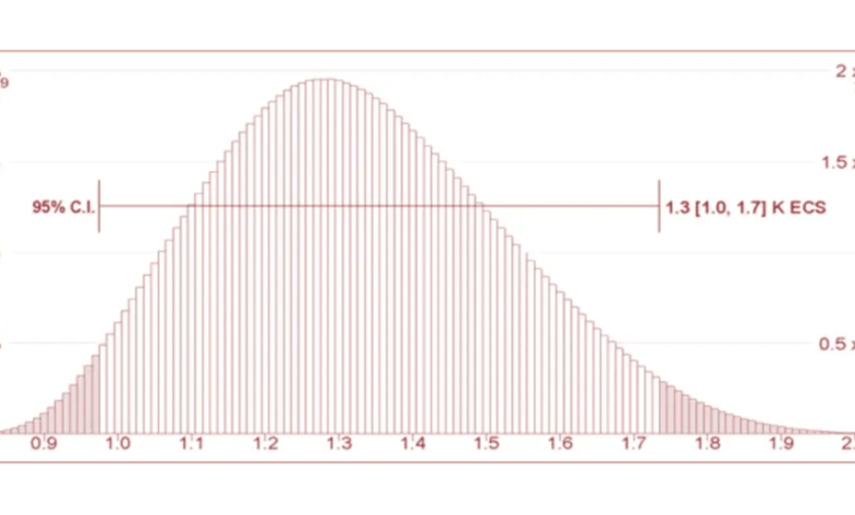
The following equation for the mid-range power budget ECS (efirst)EB. Monte Carlo simulation (109 tested) for about 2σ of a mid-range ECS of 1.3 [1.0, 1.7] K (Figure 2), which is consistent with the observed 1.4 ECS generated previously, but much lower than the 3 K expected so far.
Equation (1) assumes that the actual part of the observed industrial-period warming is due to the enforced effect (i.e. the difference between the total anthropogenic and Earth’s energy imbalance measured by satellite). Thus, the ECS is simply the product of the man-made part of the observed warming and the doubling of CO ratio.2 forced to carry out the forced industrial age. By this method, the mid-range ECS is shown to be 1.3 K, which combines nicely with the 1.4 K obtained from the previous observational method.
To verify this result, a billion-times tested Monte Carlo simulation was conducted. It produces a slightly right-skewed normal distribution as expected, producing a mid-range ECS over the period 1.3 [1.0, 1.7] K. Note that the Monte Carlo distribution is for mid-range ECS only. The upper limit can be equal to 2.1 K suggested in Roy Spencer’s paper.
The value of simple analyzes like these lies in their simplicity. Nearly all of the media has now surrendered to the climate narrative, especially out of fear Rufmord or the infamous assassination that all of us who dared to ask the “Please, sir” scientific question about that narrative have been constantly being the subject.
These simple, observational methods, especially the first, are almost understandable even to 97% of the population, who tremble at the sight of even the simplest equation. The potential influence of these simple methods on the debate becomes all the more intriguing if they are combined with a simple benefit-cost analysis.
Risk versus reward
For a number of years, the Global Warming Policy Foundation, which continues to do solid research but is not meticulously reported in the media, has been trying to find out from the Climate Change Committee. Climate change is said to be “independent” of the UK Government on how small net zero emissions of global warming will be. yield by 2050, and at what cost. The committee has been diving and diving and wriggling, but has not given a definitive answer.
However, the UK’s grid regulator has calculated that the capital cost of reconfiguring the grid to zero will cost $4 trillion by 2050; but emissions from the grid account for only one-fifth of the UK’s total emissions and operating costs (opex) are often at least double the investment costs (capex). Just ask the Germans, who during a recent cold snap (due to global warming, of course) paid $1.5 billion a week just to keep the lights on. In the UK, where coal-fired power used to cost $30/MWh, the grid regulator recently had to pay up to $11,500/MWh at a time of peak demand and these thousands of dollars in prices are increasing. It has become more frequent that coal and gas thermal energy contributions to the grid are destroyed by Government decree, leaving the grid vulnerable to collapse.
Extrapolating the Grid figures to the entire energy sector, the UK net zero investment cost would be $20 trillion, five times the investment cost of reconfiguring the grid, while operating fees will be at least $40 trillion; total costs of at least $60 trillion, which, at today’s prices, would represent three-quarters of the UK’s total GDP over the next 30 years.
Let’s now assess how much global warming the UK’s massive net zero spending will prevent. Over the past 30 years, the world’s emissions have driven an almost linear force of 1 Watt per square meter. If the whole world (let’s pretend) moves towards net zero emissions in a straight line, reducing global emissions by 1/30order emissions in 2020 each year through 2050, just over half a Watt per square meter of the next Watt per square meter of man-made force will be reduced.
Now, since one forced unit in a straight line over the past three decades has caused 0.4 K of global warming, the next forced unit halving over the next 3 decades will only prevent get 0.2 K of the next 0.4 K of warming, which the British share would be 0.002 K. Well, friends, one-fifth of a degree. At a cost of 60 trillion dollars.
On that basis, every $1 billion that the UK and the world spends pursuing net zero will only prevent 1/30 million of the warming that would otherwise have happened.
Value for money it is not. It is such simple but powerful risk-reward calculations that, as they become more known, will deservedly kill the global warming narrative.