By Frank Bosse and Nic Lewis
A recent article by Roy Spencer was (strongly) criticized by Gavin Schmidt over at “Real Climate”.
In the summary Gavin S. wrote:
“Spencer’s shenanigans are designed to mislead readers about the likely sources of any discrepancies and to imply that climate modelers are uninterested in such comparisons – and he is wrong on both counts.”
Let’s have a detailed and objective look if the wording “…to mislead the readers” is sound.
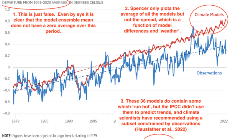
In his 1st figure Gavin S. cites a chart of Roy S. and makes remarks (in red):

Figure 1: A reproduction from the “Real Climate” article.
The annotations of Gavin are numbered, are they sound?
Point 1: Not sound. While Roy’s chart stated that the GMST-anomalies are calculated with respect to the 1991-2020 mean, it also stated that “Figures have been adjusted to align trends starting in 1979.” It is obvious from the chart that it is the multi model mean (MMM) anomalies that were adjusted to start in 1979, which is fully compatible with the pre-adjustment MMM anomalies having been calculated with respect to the mean over 1991-2020. The “This is just false” claim of Gavin S. is thus… just false. Moreover, this issue is irrelevant to the issues being studied.
Point 2: The use only of the MMM and not pointing to the model spread. Indeed: the MMM only shows the impact of the forcing (the temperature response to a given unit W/m² forcing), not the “wiggles” of single models as estimates of some internal variability. Gavin S. points to an own chart with the “spread”:

Fig. 2: A reproduction of the 2nd figure in “Real Climate” Article.
The spread shows that simulations by some models warmed no more than observations. That is consistent with Roy’s report, which said “it is generally true that climate models have a history of producing more warming than has been observed in recent decades”, and pointed out that “two models (both Russian) produce warming rates close to what has been observed, but those models are not the ones used to promote the climate crisis narrative. Instead, those producing the greatest amount of climate change usually make their way into, for example, the U.S. National Climate Assessment”. Nevertheless, the “spread” is foremost an illustration of different model sensitivities. On the basis that the real world has globally only one real TCR, the “spread” mainly represents the huge range of TCR values among different models, and this makes it of little relevance. Taking the multi-model mean enables a fair comparison between the average model’s forced warming response and observed warming, and also vastly reduces the influence of model internal variability. The actual climate system’s internal variability (“weather”) does affect observed warming (as does observational uncertainty), but over a period approaching half a century long its influence is substantially muted.
Hence this accusation of Gavin S. is unsound also.
Point 3: Gavin proposes to use a “constrained subset” of models whose TCRs were within the latest (AR6) IPCC assessed TCR “likely range” (1.4–2.2°C), which while not, as Gavin implies, being directly constrained by observations, eliminates the most-overwarming models. This is the “red zone” in Fig. 2 with a MMM as a red line. More sophisticated approaches to correcting the historical over-warming of the CMIP6 multi model ensemble, involving using observed warming as an “emergent constraint” on TCR were developed by different authors, in Tokarska et al. (2020) and Nijsse et al. (2020). Their approaches were very similar: The authors used regression to derive the relationship between TCR and historical warming across all CMIP6 models and estimated the “true” TCR from the point on the regression line corresponding to the observed warming. Tokarska et al. (2020) (T 20 in the following) thus found an ” observationally constrained” TCR best estimate of 1.70°C/2*CO2 (see Tab. S3 lower part 1981–2017 for CMIP5 and CMIP6 combined). Using a slightly different model ensemble selection, study period (1975–2019) and estimation method Nijsse et al. estimated TCR at 1.68°C /2*CO2, almost identical. These values are somewhat below the mean TCR of a screened subset of CMIP6 models with TCRs within the IPCC AR6 ‘likely range’, of about 1.75°C. In T20 the tight relation of the temperature trend slopes (If the time frame used is long enough) and the corresponding TCR is also discussed.
When eyeballing fig.2 (which includes also the huge GMST-jump in 2023) one can see that the trend slope (and hence the TCR) of the “TCR screened” MMM is slightly steeper than the observed slope. Gavin S. mentions this in his article: 0.20°C/ decade for observations; 0.23°C/decade for the screened MMM and 0.26°C /decade for the “raw CMIP6 MMM”. These relations can be used to scale TCR mean values of 1.75 found for Gavin’s “screened subset” of models, leading to a TCR (observed) of 1.52°C/2*CO2 as best estimate, almost identical to the given value in Lewis (2022). The “raw CMIP6 MMM”, scaling 1.75°C by 0.26/0.23, calculates to 1.98°C, very near the MMM value of 2.01°C given in Nijsse et al.
Conclusion for Point 3: Gavin S. is partially right, in that the CMIP6 MMM overestimates the warming to 2023 by 30%, however this was also the message of Roy S. Moreover, Gavin’s “screened subset” of models also over-warms, by 15%.
Point 4: In the following section of his article Roy S. describes the warming contrast Observations vs. CMIP6’s in the “Corn Belt summers” of the USA. For Americans this is for sure a very important region for the agriculture and save foods also in the future. Gavin S. headlines:
“Cherry-picking season”
Instead of “one small area” (CHERRY PICKING!) he recommends to plot global GISS summer trend slopes. His figure about this issue misses the point of the whole issue- it was a model-observations comparison. Therefor how well models represent the observed annual local summer (JJA) temperatures is shown here in the mentioned 1973 – 2022 time period:

Fig. 3: The correlation of the near surface temperatures 1973-2022, representing 50 years of observations, not “odd” as Gavin S. stated. Note the scale: Correlations below R= 0.5 (“by chance”) are marked in blue colors, above 0.6 in red colors. The figure was generated with the KNMI Climate Explorer.
In the “Corn Belt Region” in the USA the CMIP6 MMM has a very low performance indeed. This is also true for Australia, big Parts of South America, Central Asia, Parts of South Asia, whole Antarctica on land. The ocean performance is also weak in the East Pacific (the “pattern effect”), in the whole Southern Ocean, the South Atlantic and big parts of the North Atlantic. The region in question is not cherry picked, it’s the other way around: Looking for good matching regions with R >0.8 (i.e. West Asia, Northern South America, the Indo-Pacific warm pool) is even harder.
The point of Gavin S. is not sound.
Point 5: With his last chart Gavin S. compares the Temperatures of the lower Troposphere (TLT) from Observations and CMIP6 models:

Fig. 4: The TLT comparisons of Gavin S. He also gave the trend slopes in the caption.
It’s obviously: Two observational datasets (UAH and STAR) are generated by independent research groups and very similar. The RSS set has a much steeper (factor 1.5) trend, coming from a divergence in 2000-2006. There seems to be a problem with RSS. When one compares the likely trend slopes (0.14 for the STAR and UAH observations; 0.29 all models; 0.27 K/Dec. for selected models) as stated by Gavin S., one finds that the CMIP6 models overestimate the TLT warming (where almost all the weather is made) by a factor of about two. When the Earth’s climate is described as a coupled atmosphere-ocean-land system and one of them is so far from reality in the latest model family (CMIP6) one should not take some calculations as face value for the real world. Moreover the “screened models” seem to be adjusted only on the ground temperatures, in the TLT this adjustment method fails. This suggests problems with model physics do not relate simply to misrepresentation of feedback strength and hence climate sensitivity.
This point of Gavin S. is also not sound.
One issue remains: What is the message of Gavin Schmidt’s article? One more open question…