Guest Essay by Dr Alan Welch FBIS FRAS, Ledbury, UK — 29 June 2022
Abstract: There is a strong probability that the “accelerations” predicted by Nerem et al in their 2018 Paper (1) are due to the method of calculation and not inherent in the data. In this essay a number of data sets associated with sea level rises have been studied. The data are systematically split into a range of shorter periods and analysed using a quadratic fit in line with the method used in Nerem et al. The resulting “accelerations” and “deaccelerations” are plotted against the time period analysed in years and a power curve fitted to a plot of absolute “accelerations”.
———————————————————————-
There is a strong probability that the “accelerations” predicted by Nerem et al in their 2018 Paper (1) are due to the method of calculation and not inherent in the data. Also, in Nerem et al (2022) (2) it is stated that the “accelerations” have stabilized where in reality there has been a drop of over 10% in the 26 months since the “accelerations” peaked in Jan 2020. See “Sea Level Rise Acceleration – An Alternative Hypothesis” (3) for an essay on Nerem’s methodology. As a consequence, can anything be learnt by studying other longer sea level rise data sets in more detail?
In earlier preliminary studies of a range of sea level data some common features were noticed.
- For very long (over 100 years) the “accelerations” tended towards zero and generally were of the order of 0.01 mm/year2. Whether such low “accelerations” are actual physical accelerations, per se, or manifestations of the method of measurement or calculation is difficult to apprehend, especially if very long behaviour (over millennium) is involved.
- As time periods of analysis reduce (either due to shorter data sets or reduced period of analysis) perceived “accelerations” tend to increase.
- As well as “accelerations”, “deaccelerations” start to emerge.
- At short periods of analysis, the “accelerations” and “deaccelerations” grow rapidly and become numerically similar.
To understand all of these a common form of presentation would be useful.
The following generic presentation was devised.
- Calculated “accelerations” and “deaccelerations” are plotted against time-period covered by the analysis.
- Absolute values of “accelerations” and “deaccelerations” are plotted against time-period covered by the analysis. These are either the whole period or fractions down to 1/16th of the whole period.
- A power curve is fitted to the plot of absolute values. The choice of a power curve is appropriate in cases where there may be a relationship between two variables. The article on Wikipedia is a useful guide as to the universal suitability of this equation (https://en.wikipedia.org/wiki/Power_law). This procedure is not exactly correct as the “accelerations” and “deaccelerations” would be distributed about a long-term asymptotic value but as this may be of the order of 0.01 mm/year2 the effect would be negligible. The power curves derived are asymptotic to zero.
Below are two graphs (Figure 1) illustrating this process.
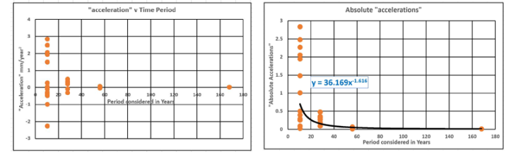
Figure 1
The first data sets studied are, together with an abbreviated reference label in parenthesis: –
The Brest Tidal Gauge data. (BREST)
The Tidal Gauge data released in 2013 by CSIRO. (CSIRO) *
The NASA Satellite data from the start 1993 to the end of 2021 for comparison. (NASA)
The 375 Tidal Gauge readings listed by NOAA. (NOAA) *
And after investigating these a further two cases were studied : –
A simulated set of data (SIM)
The Swinoujscie (Poland) data that covers 188 years (Swin).
* As these involve input from many tidal gauges over different periods care must be exercised in judging the results. For example, the tidal gauges having shorter range of dates may be the most recent and so may bias the study and conclusions.
Before proceeding with the analysis some general remarks.
In most calculations of “acceleration” use is made of quadratic curve fitting. To misquote JFK this is “not because it is difficult but because it is easy”. Any “acceleration” derived is indicative of the average over the period being considered. If the curve was a long term (millennium) variation, which in many cases is just as good a fit, the “acceleration” would be varying with time. Superimposed on top of this can be sinusoidal variations on several decade time scales. These are not part of the sea level rise but occur due to the method of measurement and the coverage.
Previous studies of the CSIRO and NASA data showed that each may contain a superimposed sinusoidal variation that causes relatively high “accelerations”. For the Tidal Gauges the underlining overall quadratic curve points to an average “acceleration” of 0.0126 mm/year2. A superimposed sinusoidal curve of +/- 6mm over a 57-year period causes additional short-term accelerations of about +/- 0.07 mm/year2 over a few years. Figure 2 below shows a combined plot against actual readings.
Figure 2
This was similar to the paper “Is there a 60-year oscillation in global mean sea level” by Chambers, Merrifield and Nerem [4]. They quoted a range of variations for oceans of between 50 to 59-year periods and a wide range of amplitudes. There was also a wide variation in phases for the different oceans so the above derived 57-year period/6 mm amplitude curve may be a reasonable average effect. Some papers suggest that the total curve can be split into a number of linear portions. See Figure 3 below taken from, Hansen et al (2015) (5). Nature would tend to smooth off such linear variations.

Figure 3
For the NASA Satellite readings there could be a sinusoidal variation about the linear best fit of +/- 3.5mm over a 25-year period that causes additional short-term accelerations of nearly +/- 0.30 mm/year2. Figure 4 below shows a combined plot against actual readings.
Figure 4
These short periods of much higher accelerations would impinge on any short periods analysed.
Figures 2 and 4 are based on my 2018 unpublished paper “Accelerating Sea Level Rise – Reconciliation of Tidal Gauge readings with Satellite Data” in which I first tried to formulate my ideas having read Nerem et al (2018).
The first 4 data sets listed above were analysed over a range of periods and graphs produced of “accelerations” and absolute values, the later also showing power curve trendlines. The 2 sets of 4 graphs are shown in figures 5 and 6.
Figure 5
Figure 6
Discussion
Brest Tidal Gauge
The total period covered by the Brest data is 211 years but due to the large gap in readings prior to 1850 only the data from 1850 to 2018 are considered. Periods analysed may vary slightly due to small gaps in the readings or where major gaps occur the affected 10.5-year periods were ignored. The “acceleration” at 168 years is 0.0108 mm/year2. At shorter periods there is a similar spread of “accelerations” and “deaccelerations”.
Apart from 1 high short period “acceleration” (investigated later) the values generally show equal levels of “acceleration” and “deacceleration”. The value of “acceleration” at the end of the trend line is 0.00994 mm/year2, very similarto the actual calculated value of 0.0108 mm/year2. The power exponent of -1.603 implies halving the time-period would increase, on average, the calculated absolute acceleration by a factor of approximately 3.
The Brest data also shows some interesting observations. As stated above the “acceleration” derived from fitting a quadratic to the Brest data between 1850 and 2018 (168-year period) is 0.0108 mm/year2. Splitting the data into 2 equal 84 year periods produces “accelerations” of 0.044 and 0.045 mm/year2 respectively. Analysing an 84-year period from 1892 to 1976, i.e. midway in the data produces a “Deacceleration” of -0.045 mm/year2. All these 3 values are roughly equal, which may be coincidental, but more importantly they are all about 4 times the 168-year value. If halving the time period can invoke such a dramatic increase in perceived acceleration what chance do even shorter periods have of giving any sensible values. These analyses are shown in Figure 7.
Figure 7
It was also pointed out that there was one “acceleration” over a period of 10.5 years that was much higher. Around 1912 the sea levels were recorded as extra high and the 10.5 year period covering 1912 had this higher sea levels at one end. As a result the “acceleration” derived was 6.04 mm/year2, over 500 times the 168 year result. Moving the period covered on by 4 years causes the high “acceleration” to become a high “deacceleration” of 7.56 mm/year2 as shown in Figure 8. This indicates how short periods can totally distort any “acceleration” estimations. Imagine extrapolating either of the 2 curves in Figure 8 for 100 years. The sea would rise over 36m or fall over 39m!

Figure 8
CSIRO Data
The next study involves the Tidal Gauge results the data for this having been extracted from an earlier version of the https://climate.nasa.gov/vital-signs/sea-level/ site and referenced to CSIRO as its source. The data file extracted from the CSIRO source was labelled “CSIRO_Recons_gmsl_mo_2015” and can be obtained by googling this name. This covered the period from the beginning of 1880 to the end of 2013 and again a range of periods were used to ascertain “accelerations”.
The power exponent of -0.473 implies halving the time period would only increase the absolute acceleration by 30%. Possibly because many tidal gauges are combined this may smooth out the curve.
NASA Satellite Data
Even though the Satellite readings only cover a small (less than 30 years) period a similar exercise was performed.
Interestingly the trend line at about 29 years reads only 0.0179 mm/year2 much less than the 0.0884 mm/year2 predicted by the quadratic fit to the complete data. Also, the exponent value of -2.001 implies halving the time-period quadruples the acceleration derived. Calculating the “acceleration” at 2050 (57 year period) and 2100 (107 year period) yields “accelerations” of about 0.0046 and 0.0013 mm/year2. These values should be treated with caution and only indicative of how fast “accelerations” can drop in the long term.
375 NOAA Tidal Gauges
The 4th study is slightly different as it analyses the 375 Tidal Gauge readings listed in NOAA’s “2016 list of 375 long term trend tide stations” (6). These cover varying time periods from 28 years (Santa Cruz, Ecuador) to 209 years (Brest, France).
All “accelerations” above 150 years are less than 0.02 mm/year2.
All “accelerations” above 100 years are all less than +/- 0.06 mm/year2 and mainly less than0.03 mm/year2.
The value of the exponent of -2.12 implies the absolute acceleration would increase by a factor of 4.3 if the period analysed is halved but as each value is a separate tidal gauge not so much should be read into this. It is the similar behaviour that is of interest.
General
There is a commonality to the forms of the “accelerations” and a consistency in the power term in the trend lines of around -2.0 +/- 0.4. What could cause this? Possibly the sea levels, or more accurately the sea level data, are created by several sinusoidal responses that could cover the smaller decadal oscillations up to any long term (millennium) periods.
Before investigating this the Brest results were looked at in a different way. The absolute “acceleration” curves and associated power curves were investigated as though there were only results for the first 84, 56 or 42 years. The results of this are shown below in Figure 9 along with the 168-year case. The power curves were extended to 168 years and the values of “acceleration” at 168 years are also shown for each period considered. They all lie within the range of about 0.015 +/- 0.005 mm/year2.
Figure 9
The value of the “accelerations” at 168 years are calculated from the Power Curves and gives the following when compared with the value obtained with the quadratic curve over the full 211 Years.
From “acceleration” Number of data points
211 years 0.0108 mm/year2 Used 1886 data values
168 years 0.0099 mm/year2 38 “acceleration” estimates
84 years 0.0170 mm/year2 19 “acceleration” estimates
56 years 0.0187 mm/year2 13 “acceleration” estimates
42 years 0.0098 mm/year2 8 “acceleration” estimates
Simulated Data Set
Having analysed these 4 data sets, an investigation of an artificial data set was produced that involved 4 sinusoidal curves of 1000, 333, 177 and 89-year periods with amplitudes of +/- 400, 250, 160 and 90 mm respectively these being variations about a linear increase. The total 1000-year curve is shown below in Figure 10. This is not a random curve but is not atypical of long-term behaviour.
Figure 10
The “accelerations” would be the same if calculated from this curve or the residual curve shown in Figure 11.
Figure 11
A final study of this curve was made calculating the “acceleration” over the whole 1000 years, then in portions of two 500 years, four 250 years and eight 125 years.
Plots of “accelerations” and “deaccelerations” and absolute “accelerations” are plotted in line with previous studies. (Figures 12)
Figure 12
The graphs show the same form as in the other 3 studies and the power term is -1.99, close to the -2 value. Perhaps this value of -2 is an outcome of using sinusoidal variations.
Swinoujscie (Poland)
As a further study another long data set , from 1811 to 1999, was analysed in the same way and this produced the plots in Figure 13 showing a power coefficient of -2.481.
Figure 13
The “acceleration” over 189 years is 0.0106 mm/year2. Halving the time period results in values of 0.0272 and 0.0136 mm/year2 whilst the quarter ranges give -0.0524 to 0.0162 mm/year2. Using ranges of about 24 years results in a dramatic rise in the values of “accelerations” from -0.59 to 0.32 mm/year2.
Conclusions
Overall, the main conclusion points to the NASA time range of nearly 30 years being much too short to predict the “accelerations” and therefore any extrapolation may be totally unrepresentative of future long-term behaviour. Extending the power curve for the NASA readings to 2050 and 2100 points towards a much smaller long term “acceleration” of the order of 0.01 mm/year2 in line with many long-term studies.
Also, the analyses show that even over periods greater than 100 years the calculated “acceleration” could still be reducing because of Decadal Ocean Oscillations and methods of measurement, including the fact that 100% coverage is not possible. At shorter periods the abundance of “accelerations” and “deaccelerations” tends to become similar.
Curve fitting should not be ruled out as an aid to understanding data but polynomial curves can be misleading near the ends of the data range.
It is also difficult to judge what is an acceptable time range that may give meaningful predictions. In some tidal data 100 years is still insufficient. Satellite data may be more accurate but it still early days to judge behaviour let alone predict the future.
References
- Nerem, R. S., Beckley, B. D., Fasullo, J. T., Hamlington, B. D., Masters, D., & Mitchum, G. T. (2018). Climate-change-driven accelerated sea-level rise detected in the altimeter era. Proceedings of the National Academy of Sciences of the United States of America, 115(9). First published February 12, 2018
- Nerem, R.S., Frederikse, T, Hamlington, B. D. (2022). Extrapolating Empirical Models of Satellite-Observed Global Mean Sea Level to Estimate Future Sea Level Change. AGU Advancing Earth and Space Science. https://doi.org/10.1029/2021EF002290. First published 21 March 2022.
- https://wattsupwiththat.com/2022/05/14/sea-level-rise-acceleration-an-alternative-hypothesis/
- Chambers, Merrifield and Nerem (2012). “Is there a 60-year oscillation in global mean sea level?” https://acp.copernicus.org/preprints/15/20059/2015/acpd-15-20059-2015.pdf
- https://agupubs.onlinelibrary.wiley.com/doi/pdf/10.1029/2012GL052885
- http://sealevel.info/MSL_global_thumbnails5.html
# # #