By Ad Huijser
After reading “Into The Black Box” (ref. 1), once again a great and very informative contribution by Willis Eschenbach, I wasn’t so much surprised by the conclusion that a “one-liner climate model” could generate a result similar to that of the most complicated GCM’s. However, I was puzzled that he stopped his analysis there. The recurrent relation he applied, between temperature change and forcing, is a straightforward consequence of how the surface temperature T
So, let’s look somewhat closer to this recurrent relation that I will (provocatively) refer to as CMC: the Climate Model Checker. If n-1, n, n+1 are consecutive times at unit time intervals we can easily derive this relation for small perturbations in the energy in- and outflows of the Earth climate system from the energy balance according to C ∂T/∂t = “Radiation IN” – “Radiation OUT”, as:
Tn+1 = Tn + λ (Fn+1 – Fn)(1 – exp (-1/τ)) + (Tn -Tn-1) exp(-1/τ)
in which τ is a specific response time primarily determined by the heat capacity C of the Earth’ climate system and λ a factor representing the climate sensitivity, the way in which the surface temperature T responds to an imbalance F at TOA. It’s obvious that λ = ∆T/F where ∆T is the surface temperature increase for t®µ , due to a step-wise forcing F at t = 0. This sensitivity can be related to the temperature rise due to the forcing of doubling of the CO2 concentration, the well-known Equilibrium Climate Sensitivity expressed as ECS = λ F2xCO2.
One might argue that I have just shifted the problem to estimating the parameters λ and τ, and thus to the ongoing discussion “what is the value of ECS?”. True, but first of all, we now have only 2 parameters to adjust rather than the large set of parameters/estimates in any complicated GCM. And secondly, we can begin by just using what seems reasonable and see where we get from there.
First, we have to estimate a realistic value for τ. For a water planet and based on the choice of the depth of the mixed ocean layer, textbooks (e.g. ref. 2) arrive at about 4-5 years. With 1/3 land, that value will probably be not much lower than 3 years. An average of 4 years will be a good estimate and is supported by Willis’ analysis of τ = 4.2 in fitting this CMC to the CMIP5 ensemble (ref. 1). In practice, this CMC happens to be not very sensitive to response times in the interval of 3 to 5 years.
Next, we need an estimate for the climate sensitivity λ. As a starter, I go blindly for the inverse of the Planck feedback parameter of 3.3 W/m2/K (don’t bother about +/- signs here) as it is derived from the same origin as our CMC, and equal to 4(1-a)Φ0/TS0, with the all sky albedo a = 0.3, the average solar incoming radiation Φ0 = 340 W/m2 and the equilibrium surface temperature TS0 = 288 K. So, λ = 0.3 K/ W/m2 would be an excellent choice, and indeed Willis’ analysis (ref. 1) of best fits to the CMIP5 outcomes, is showing values close to that.
But these values didn’t fit well the Berkeley temperature series where he needed λ = 0.4 K/ W/m2 and τ = 5 years. Now we all know: the output of models is a “translation” of the input, or in short: “what you put in, you get out” (but don’t forget: “what you don’t put in, you cannot get out”). So, the question arises, is this difference between the Berkeley, and this CMC calculated temperature range due to the wrong choice of λ and τ, or an effect of the chosen “input”, i.e. the time dependent forcings?
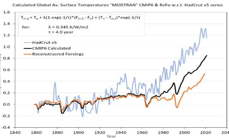
To find out, I downloaded Eschenbach’s Excel spread sheet and constructed my own accordingly. To test mine, I used the same CMIP5 input from the NASA/GISS site (ref 3). Instead of the Berkeley temperature series, I used the most recent HadCrut v5 (ref 4) series as being more “current”, to compare with. What became quickly clear is that with λ = 0.3 K/W/m2 and τ = 4 years, this CMC fits reasonably well to the HadCrut v5 temperature series. But with a slight increase to λ = 0.345 K/W/m2 it even fits excellently. This somewhat higher value for λ is not based on curve fitting, but comes from the simulations with the on-line MODTRAN module from the University of Chicago (ref. 5) for the US Standard Atmosphere + clouds (Stratus/Strato CU) + Relative Humidity taken 1 and “constant”. Since it doesn’t change any conclusions, and as I will also use some outcomes of MODTRAN under those particular conditions further on in this essay, I will use this higher λ value for practical/consistency reasons from now on.
This fit is shown in fig. 1a and in fig. 1b the same fit is show with the UAH LT temperature series (ref. 11), which is unfortunately only available for the last 40 years. To better show the warming trend, I used the option to suppress the volcano contribution to the total forcing (dashed lines).
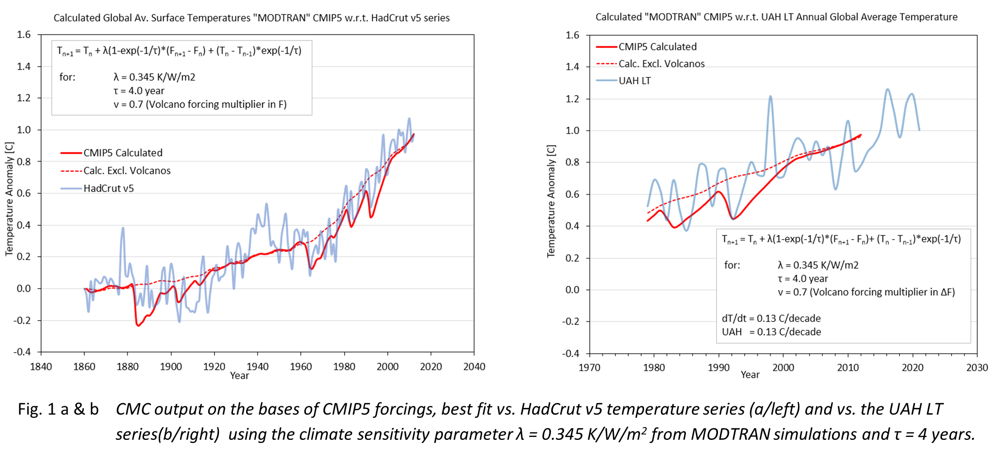
Clearly, not bad at all, but no news given Willis Eschenbach’s earlier analysis (ref. 1), and I leave it to others to explain the enormous discrepancies between this CMC and measured temperatures around 1940 (hot WWII times?), apparently not due to any known anthropogenic forcing.
But downloading the CMIP5 forcings from the GISS website (ref. 3), I noticed also the availability of the CMIP6 database. Expecting it to be more actual, I tried those forcings as well (don’t know why Willis didn’t use this set). Anyhow, what came out of applying these CMIP6 inputs to the same CMC calculation with the identical λ and τ parameters, was a complete surprise as fig. 2 shows. And here, the remark that “the models’ output is always a reflection of the input”, makes clear that the CMIP6-models input is completely different from the CMIP5 input data, as shown in fig. 3. And not just by a small fraction; a forcing difference of 1 W/m2 in 2010 on an average of 2.5 W/m2 is simply outrages.

One could expect some new insights in the category “natural forcings”, but not in the forcings from the category of the well mixed greenhouse gasses (WMGHG). As both input data are from the same group of people with supporting literature (ref. 6), I searched in there for new insights or good arguments for these discrepancies. They Indicated some differences, but without clear explanations. Maybe my shortcoming, but I couldn’t find one serious discussion for their choices. But reading the following statement on their website (ref. 3) gives me the impression that they allow themselves the option to adjust anything they see necessary to tune the input to the output:
“Quantifying the actual forcing within a global climate model is quite complicated and can depend on the baseline climate state. This is therefore an additional source of uncertainty. Within a modern complex climate model, forcings other than solar are not imposed as energy flux perturbations. Rather, the flux perturbations are diagnosed after the specific physical change is made. Estimates of forcings for solar, volcanic and well-mixed GHGs derived from simpler models may be different from the effect in a GCM. Forcings from more heterogeneous forcings (aerosols, ozone, land use, etc.) are most often diagnosed from the GCMs directly”.
IPCC’s AGW-narrative is partially based on the claim that all these GCM’s can adequately replicate the warming since the pre-industrial period. It’s clear now that such claims are not about climate models, but about models+input. Where the CMIP5 models+input could be covered well with λ = 0.345 K/W/m2, the CMIP6 models+input needs a value of 0.555 K/W/m2 (fig. 4). And obviously, this “extra” 0.21 K/W/m2 climate sensitivity, is not model-, but input related. So, discussions on the change in climate sensitivity between CMIP5 and CMIP6 ensembles, are in fact useless, unless models and input are clearly decoupled and models are compared with the same set of forcings as input. It is too easy to speculate that this is proof of “tuned” input, but this issue anyhow asks for a better insight into the forcings applied in these ensembles. So, I tried to understand the CMIP6 composition in more detail as it has the lowest WMGHG-contribution, as depicted in fig. 3 & 5.
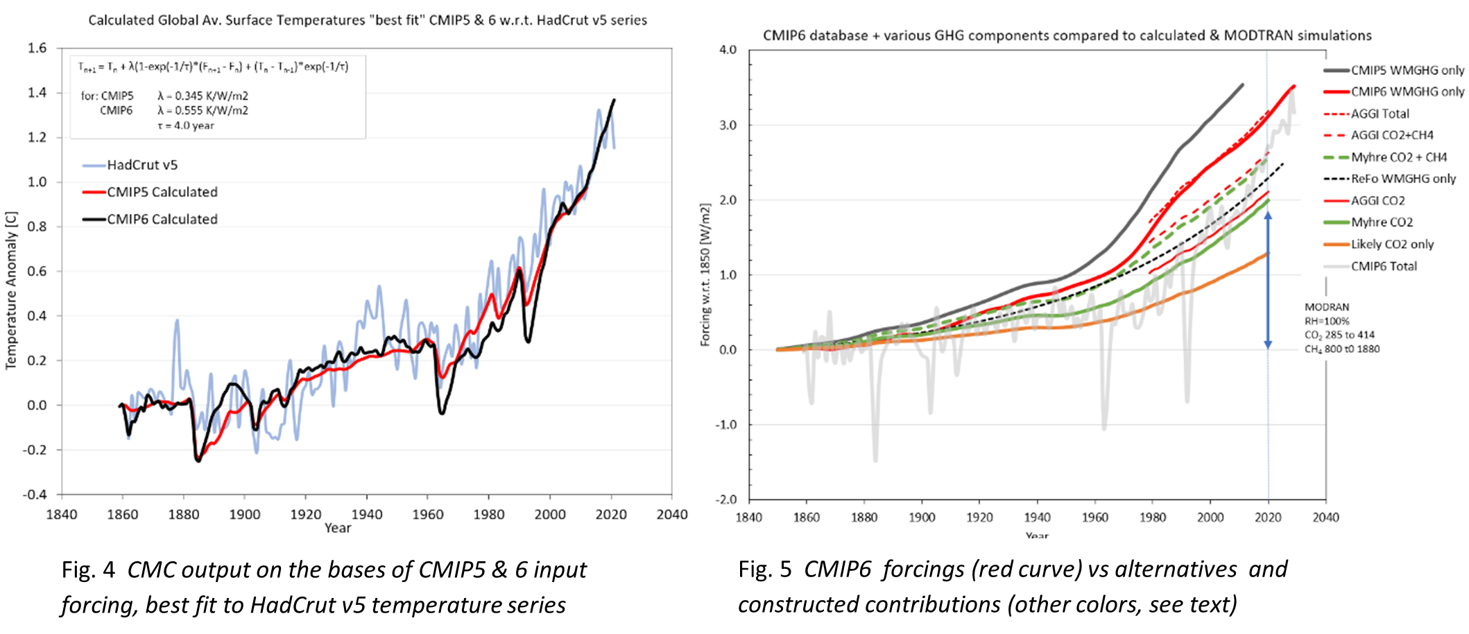
In the downloadable CMIP6 database, all GHG’s are clustered into one WMGHG forcing and to decompose this, I made use of AGGI, the NOAA Annual Greenhouse Gas Index data (ref. 7) which goes back to 1979 (thin/red curves in fig. 5). Their total WMGHG (red dotted line) fits well with the CMIP6 data, but not at all with the CMIP5 input (black line). There are 4 major contributors, CO2 (solid thin red), CH4 (on top of CO2, dashed thin red) and the “rest” from NO2 and CFC/HCFC’s. The steep rise in forcing after 1970, is apparently caused by the latter 2 components, but it is difficult to imagine that they contribute almost all of a sudden about 1 W/m2 to the total forcing. Nevertheless, CMIP6 forcings are consistent with these AGGI data over the available period, so they are probably “objective” assessments from GHG-concentration changes in the atmosphere.
What we can easily check in that context, is the contribution of Carbon Dioxide and Methane. Here, the MODTRAN module is a handy tool as it allows to reconstruct the forcings for both CO2, being the largest contributor and Methane (CH4) as “runner up”. To do so, we just need the concentration of these GHG’s since the pre-industrial era. For CO2, that’s not a problem, as we have the Mauna Loa data plus the Carbon Project with long-time “best estimates” for historic fossil fuel emissions and the reconstructed 280 ppm in 1850 seems undisputed. For Methane the history is less clear. We have since 1984 reliable measurements, but Methane sources are pretty speculative, primarily coupled to the growth of the global population and the coupled growth in agriculture and the amount of cattle. The pre-industrial concentration (about 800 ppb in 1850) comes from analyzing trapped air in ice cores. How reliable those data are, is questionable. Although I modeled the known concentrations back to about 1100 ppb in 1850 using recent emission rates and a 9 years lifetime, I have no reason to reject this “official” value of 800 ppb and use it to calculate the CH4 forcing. If we use MODTRAN to simulate the effect of going from the 1850 CO2 and CH4 concentrations to today’s levels (414 ppm and 1880 ppb, respectively), we arrive at 1.85 W/m2 total forcing for the US Standard Atmosphere with Stratus/Strato CU-clouds, and the Water Vapor setting at 1 and at constant RH. The latter simulates “water vapor feedback” (WVFB), the effect of a changed H2O concentration due to temperature changes, so no need to have any discussion later on, on that controversial issue.
This total “MODTRAN” CO2+CH4 forcing, indicated in fig. 5 by the blue arrow, immediately questions the credibility of the NASA/GISS forcings used in the CMIP5 & 6 databases. The forcings used in the AGGI database seems to be based on the work of Myhre et al (ref 8) from which we immediately recognize the use of the well know 2xCO2 forcing value of 3.7 W/m2 and CH4 forcings from the same study (green solid and dashed curves). However, we know from the recent work of Van Wijngaarden and Happer (ref. 9), that the specific CO2 forcing is certainly too high and 3.0 W/m2 at max, since they determined it for clear sky conditions only. The MODTRAN module yields for that situation F2xCO2 = 2.95 W/m2, in good agreement with their work. But for the all sky (cloudy) conditions, as applied throughout this work (and including WVFB), this value drops even to 2.26-2.36 W/m2 (depending on the RH value between 100-60%) since clouds partially shield off the effect of GHG’s. To illustrate in fig. 5 the difference this makes, I included the “Likely CO2 only” curve with 2.4 W/m2 (orange curve).
The NO2 contribution in the AGGI is not more than 0.2 W/m2, so the steep rise in forcings must be due to the ChloroFluorCarbon’s. In MODTRAN, these are represented by the Freon Scale, and toggling that between 0 and 1, yields only 0.09 W/m2 of extra forcing for those gasses.This low value is difficult to match with the about 0.5 W/m2 forcings indicated by the CMIP6 and AGGI data.
Anyhow, the total forcing difference of the WMGHG’s CO2 + CH4 + NO2 + CFC’s, between 2020 and 1850 will certainly not be more than 2.3 W/m2 according to the numbers above; considerably lower than the 3.2 W/m2 as being used in the CMIP6 database from NASA/GISS. And I see absolutely no reason to doubt about my accounting, nor see any option to bridge this gap of almost 1 W/m2.

Of course, we could try to fix this discrepancy by adapting the climate sensitivity λ and/or the response time τ. But that doesn’t make much sense as we have to go to at least 1 K/W/m2. This would imply a ridiculously high climate sensitivity (according to ECS = λ F2xCO2 ≈ 3 K) although still within the IPCC range or, in GCM’s terminologies, an indication for absurd high feedbacks. The latter is exactly the excuse of CMIP6 models and the background to the recent CMIP6 based alarmistic conclusions of even higher future warmings than forecasted before. And what I show here with this CMC calculation for both the CMIP6 and the REFO set is, that where the CMIP5 models + input can apparently fit the measured temperature series between 1850-2020 reasonably well, the CMIP5 & 6 models + objective input (as this REFO) don’t fit at all.
So, this gap between the anomalies calculated from forcings and what is observed will be difficult to bridge by anthropogenic driven effects. My own assessment (ref. 10) is that the change in cloud-cover since 1980 can do that job, when accepting a climate sensitivity to cloud-change of about -0.11 K/%cc rather than the awkwardly high positive cloud-feedbacks due to temperature increase in GCM’s. It’s amazing that MODTRAN, contrary to GCM’s, also gives a similar answer to that question but that’s “another story”, and not for this context to address. But keep in mind, the observed cloud change might not be the only effect influencing global climate change, so we have to keep our minds open to other options as well.
In conclusion: I have tried to analyze in a transparent way the quality of GCM climate models and whether the AGW-hypothesis is well proven by these models over the period 1850-2020, as the IPCC claims they do.
After this exercise, the only answer I can come up with is “no, absolutely not !”. Models that need model-specific input to replicate the known past, violate the most basic criteria of science to earn the label “scientifically proven”, independent of the “proven physics” they are based upon. These models are indeed “Black Boxes” but without any predictability. The striking inconsistencies in input values between the various generations, should already be sufficient reason to reject any outcome. And consequently, these models are totally, in all aspects, inept to forecast the future.
The question: “are these CMIP5 and CMIP6 forcings fixed to the temperatures of the last 1½ century to fit the respective GMC-models’ predetermined/wishful outcome”, remains unanswered as I have no insights in how GMC’s are actually tuned. But this analysis coupled to the earlier quote from the NASA/GISS website, leaves that option clearly open.
This conclusion doesn’t make me a climate denier or an advocate to go on polluting, but the idea that global warming could be influenced if not stopped, by massive CO2 reductions, is to my opinion not supported by proper scientific evidence.
With thanks to Willis Eschenbach for triggering me to make this analysis.
Ad Huijser February 20, 2022
References
- Eschenbach, https://wattsupwiththat.com/2022/02/03/into-the-black-box/
- See for instance: http://www.atmos.albany.edu/facstaff/brose/classes/ATM623_Spring2015/Notes/Lectures/Lecture02%20–%20Solving%20the%20zero-dimensional%20EBM.html
- https://data.giss.nasa.gov/modelforce/
- https://www.metoffice.gov.uk/hadobs/hadcrut5/
- http://climatemodels.uchicago.edu/modtran/
- Miller et al, 2014, CMIP5 historical simulations (1850-2012) with GISS ModelE2, Journal of Advances in Modeling Earth Systems, vol. 2, 441-468 https://doi.org/10.1002/2013MS000266 and
Miller et al, 2021, CMIP6 historical simulations (1850-2014) with GISS-E2.1, Journal of Advances in Modeling Earth Systems, vol. 13
https://doi.org/10.1029/2019MS002034 - https://gml.noaa.gov/aggi/aggi.html
- Myhre et al, 1998, New Estimates of Radiative Forcing due to Well Mixed Greenhouse Gasses, Geophysical Research Letters, vol 24, 2715-2718
- W.A. van Wijngaarden and W. Happer, Relative Potency of Greenhouse Molecules, arXiv:2103.16465v1, 30 Mar 2021
- Huijser, The under estimated role of Clouds, https://www.clepair.net/clouds-AdHuijser.pdf
- https://www.nsstc.uah.edu/data/msu/v6.0/tlt/uahncdc_lt_6.0.txt