
If you have a call center and track incoming callers and their call duration, you can store all that information in Microsoft Excel. The sheet will store the caller identifier and timestamp values.
However, reporting them won’t be as simple as printing out a list each day since callers can call multiple times in a day. That’s what will mean for those who need the information.
In this tutorial you will learn what a timestamp is and then how to use the MIN() and MAX() functions in Excel to return the first and last call of the day from the timestamp. You would then create a clustered set of records that return the first and last call for each caller.
I am using Microsoft 365 on Windows 10 64-bit system. Some of the functionality used is only available in Microsoft 365 and Excel for the web. Friend download demo for this Excel tutorial.
UNDERSTAND: Windows, Linux, and Mac commands everyone needs to know (free PDF) (TechRepublic)
How to return value for the first time in Excel
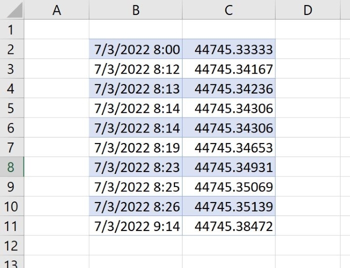
A timestamp is a combined date and time that marks a specific time. If you change the cell’s format to General or Number, you’ll see a number instead of a date. The integer of the number represents the date and the decimal value represents the time of the day.
For example, Picture A displays a timestamp column formatted to display as a date and time. The column next to it shows the underlying values for each timestamp.
Picture A
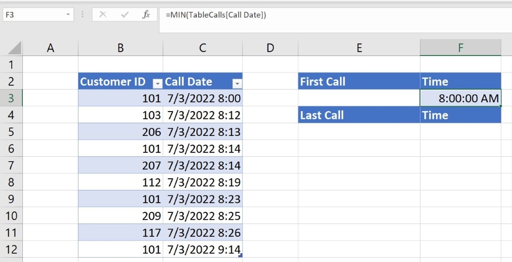
Now, let’s say your helpdesk call center keeps track of the caller’s call and the time it came in. At the end of the day, you want to know the first and last call of the day. A simple illustrated table is shown in Figure BUG lists the calls in order, so it’s easy to see the first and last calls, but not always, depending on how the employee entered the call records.
Figure BUG
It would be very easy for an operator to enter a call record a few minutes later than it was received, and then your records would be out of order, over time. So we won’t take that into account in our solution.
Fortunately, Excel’s MIN() function returns the earliest call (smallest time value) of the day. This simple function requires only one argument, and that is the scope or structured reference containing the values we are evaluating.
Function
= MIN (TableCalls[Call Date])
use a structured reference because the data range is an Excel Table object named TableCalls. If you were evaluating a normal range of data, you would use the reference
= MIN (C3: C12).
Function
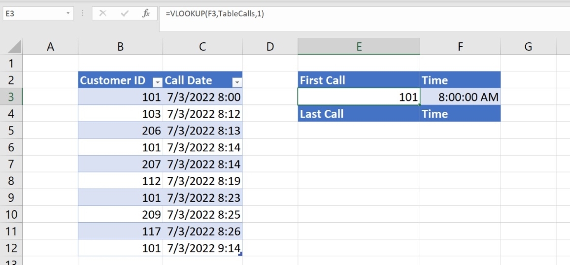
= VLOOKUP(F3, TableCalls, 1)
returns the customer that made that first call, as shown in SIZE. Structured reference, TableCalls is the name of the Table. F3 refers to the time of the first call (on the right), and argument 1 returns the corresponding value in the first column of TableCalls.
SIZE
Now let’s go back to the last call of the day.
How to return the last time value in Excel
After working through the functions to return the earliest call and the client to make that call, doing the same for the last call of the day was simple. We will use the MAX() function to return the last call and another XLOOKUP() function to return the client that made that call.
Visualization show both functions:
E5: = VLOOKUP(F5, TableCalls, 1)
F5: = MAX(TableCalls[Call Date])
Visualization
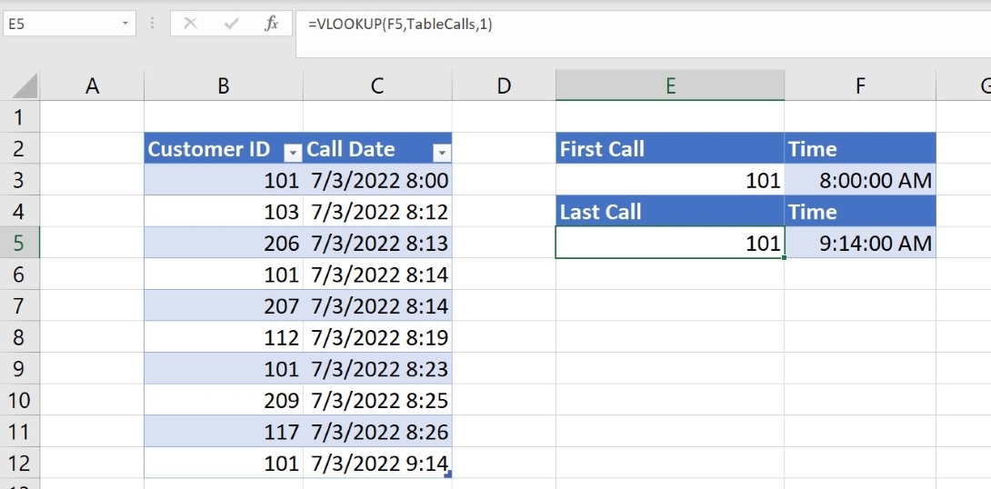
The XLOOKUP() function returns the client that made the last call by finding the time value in F5 and returns the corresponding value from the customer ID column. The MAX() function returns the latest call (maximum time value) from the time values in the Call Date column, C5:C12.
If you’re tracking and the time values in F3 and F5 are showing both the date and time, you can reformat those cells to show only the time.
First, select F3, and on the Home tab, click the Format drop-down menu in the Number group. Select Time from the drop-down list. Repeat these steps for cell F5.
That’s easy and works if all you need is the first and last call of the day. Let’s say you want a record for each customer that returns the first and last call of the day if that customer makes more than one call. This requirement is more complicated.
How to return a caller and their calls in a record in Excel
Maybe management wants to see a list of all customers with their first and last calls if that customer makes multiple calls. You won’t meet that requirement with a few simple functions, but you can (Figure E).
Figure E
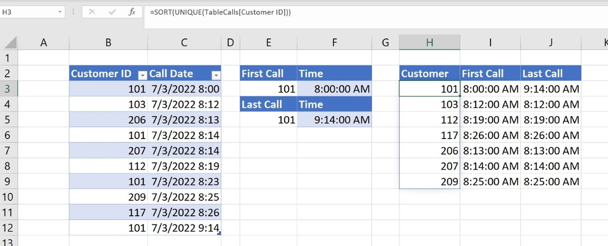
The first step is to return a list of unique customer IDs. To do so, enter the following dynamic array function in H3
= SORT(ONLY(TableCalls[Customer ID]))
This function returns a list of unique customer ID values sorted as a dynamic array. That means there is only one expression and it is in H3. The rest of the column is the overflow range - the result needed to execute the expression.
To return the first call for each customer ID, enter the following function in I3 and copy it into the remaining cells:
= XLOOKUP($H3, TableCalls[Customer ID]TableCalls[Call Date])
This function returns the first call for the corresponding customer ID in column H.
To return the last call for each customer ID, enter the following function in J3 and copy it into the remaining cells:
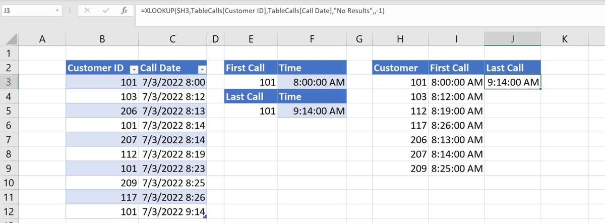
= XLOOKUP($H3, TableCalls[Customer ID]TableCalls[Call Date]”No results” ,, - 1)
The last argument, -1, does a bottom-up search, that’s why it can return the last call. If you sort your calls in descending order, you’ll need to modify both functions by removing it from the function in J3 and adding it to the function in I3.
This setup works, but only one client is called more than once, so the functions will copy the first call to the last. The result is worse than distracting, it’s confusing, so add a conditional formatting that will hide duplicates in the last call column.
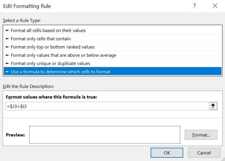
First, select J3:J9 and on the Home tab, click Conditional Formatting in the Styles group and select New Rule from the drop-down menu. In the resulting dialog, click the last selection in the top pane, Use Formulas to Determine Which Cells to Format.
In the formula control, type = $J3 = $I3 (Figure F). Click Format, click the Font tab, choose white from the palette, and click OK twice to return to the sheet.
Figure F
As you can see in WOOD Figure, only the last value for customer ID 101 is displayed. The other values are there, but you can’t see them because the font is the same color as the background. I don’t like hiding things, but since this will update frequently it seems like a convenient solution.
WOOD Figure
Keep stable
It seems like a lot of work, but all the functions we used were easy to implement. One glitch is that you can’t use dynamic array functions in Table objects. That means you have to update the functions in columns I and J and conditional formatting references, as needed. For that reason, I’ll show you how to do the same thing with a PivotTable in a future article.
If you are new to XLOOKUP(), you can read How to use the new XLOOKUP() dynamic array function in Excel. To learn more about UNIQUE(), read How to use UNIQUE() function to return count of unique values in Excel.