Guest Post by Willis Eschenbach
In my most recent post, titled “Where is the top of the atmosphere?“, I used what is known as “Ordinary Least Squares” (OLS) linear regression. This is the standard type of linear regression that gives you the trend of a variable. For example, here is the OLS linear regression trend of CERES surface temperatures from March 2000 to February 2021.
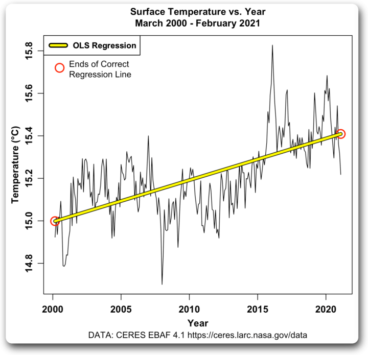
Figure 1. OLS regression, temperature (vertical or “Y” axis) versus time (horizontal or “X” axis). The red circles mark the endpoints of the correct regression trendline.
However, there is an important announcement about OLS linear regression that I am not aware of. Thanks to someone knowledgeable about statistics comment In my last article, I discovered that there are several things that must always be considered regarding the use of OLS linear regression.
It only gives the correct answer when there is no error in the data displayed on the X-axis.
Now, if you’re looking at some variable on the Y-axis versus time on the X-axis, this shouldn’t be a problem. Although there is often some uncertainty in the values of a variable such as the average global temperature shown in Figure 1, in general we know the timing of the observations fairly accurately.
But suppose, using exact same data, we put time on Y axis and temperature on X axis and use OLS regression to get trend. This is the result.

Figure 2. OLS regression, time (vertical or “Y” axis) vs temperature (horizontal or “X” axis). As shown in Figure 1, the red circles mark the endpoints of the exact regression trendline.
YES! That’s the way, the wrong way. It greatly underestimates the true trend.
Fortunately, there is a solution. It’s called “Deming regression” and it requires you to know the errors in both the X and Y axis variables. This is Figure 2, with the Deming regression trendline shown in red.

Figure 3. OLS and Deming regression, time (vertical or “Y” axis) vs temperature (horizontal or “X” axis). As shown in Figure 1, the red circles mark the endpoints of the exact regression trendline.
As you can see, Deming regression gives the correct answer.
And this can be very important. For example, in my previous post, I used OLS regression in a scatterplot that compares the uppermost layer of the atmosphere (TOA) long wave (Y-axis) with the surface temperature (X-axis). The problem is that both TOA enhanced LW and temperature data have errors. Here is the plot:
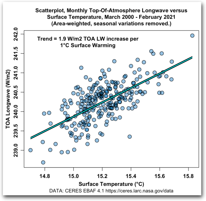
Figure 4. Scatter plot, monthly top-atmospheric longwave (TOA LW) versus surface temperaturee. The blue line is an incorrect OLS regression trendline.
But that is incorrect, because of the error in the X-axis. After the commenter pointed out the problem, I replaced it with the correct Deming regression trendline.

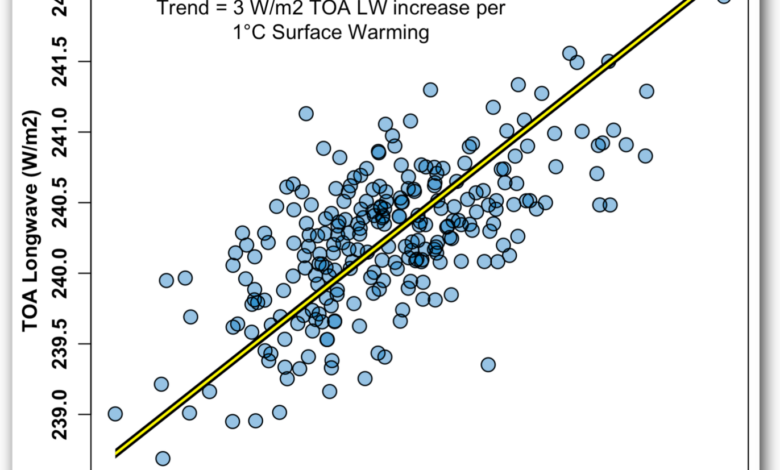
Figure 5. Scatter plot, monthly high-level long wave of the atmosphere (TOA LW) compared with surface temperature. The yellow line is the correct Deming Regression trendline.
And this is quite important. Using the incorrect trend shown by the blue line in Figure 4, I miscalculated the equilibrium climate sensitivity of 1°C for a doubling of CO2.
But use the right trend shown by the blue line in Figure 5, I calculate an equilibrium climate sensitivity of 0.6°C for a doubling of CO2…a significant difference.
I love writing for the web. No matter what topic I choose to write about, I can guarantee that there are people reading my posts who know more than I do about the topic in question… and as a result, I’m constantly learning new things. It’s the world’s best peer-reviewed.
I thank the commenter for putting me on the right path and I extend my best regards to all,
w.