By Charles Blaisdell PhD ChE
- Abstract
The earth’s seasonal oscillations in cloud cover are related to global changes in evapotranspiration, ET, from the earth’s tilt and more land surface in the Northern Hemisphere. This paper presents a simple model that explores the climate change possibility of changing the Land ET over the years.
Evapotranspiration, ET, is the Earth’s combination of Evaporation and plant Transpiration of water. It has long been assumed that the Earth’s ET and cloud fraction did not change much over time (years). Resent data has shown that anthropic land changes can cause regional ET reduction[15] and [16]. (These ET changes are from what the ET is now vs what the ET of the same land would have been if the anthropic change were not made.) Resent data has also observed cloud fraction reduction over the last 45 years [5]. This paper presents a mathematical model that shows the relationship between Anthropic land related ET change and Cloud Reduction (and Increase). The Model creates one anthropic Special Parcel of land that represents all anthropic land changes like Urban Heat Islands, UHI’s, forest to cropland, mining, etc. that can have ET change over time. The Model steps through the natural water cycle of this Special Parcel and the whole Earth: 1) The Special Parcel has a decreased Evapotranspiration, ET, vs its natural state and this decrease in ET (on average) will result (using proven vapor pressure equations) in air rising from this Special Parcel to have increased temperature and lower relative humidity. 2) This higher temperature and lower relative humidity air rises to where lower clouds (cumulus) form in a plume equal to or greater than the area of the Special Parcel. 3) The plume from this special parcel mixes with the rest of the atmosphere at cloud elevation and results in a small increase in temperature and lower relative humidity (calculated at ground level). 4) Higher temperature and lower relative humidity reduce the probability of cloud formation (or lower cloud density/reflectivity). 5) Less Clouds more sun. 6) More Sun, the hotter it gets and the more evaporation (some increase in Transpiration too), global ET increases. See Figure 1. This is how a reduction in ET (local) will cause an increase in ET (global). Another view: The Special Parcel over time has lowered the water put into the atmosphere that would have made clouds, less clouds more sun.
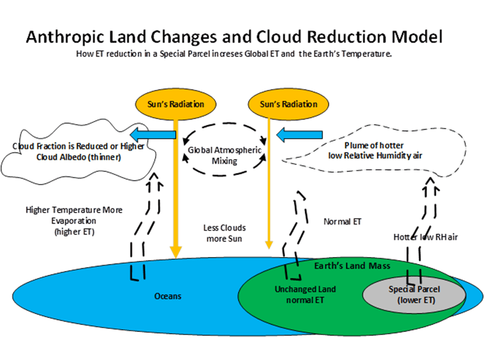
The Special Parcel variables in the Model are: 1) How much ET change occurs in the Special Parcel area. 2) How big is the Special Parcel. 3) How big is the air plume. The Model shows that current possible range of these variables could possibly account for a significant part of the observed Global Warming, GW.
The Model uses Clausius–Clapeyron related equations in Psychometric charts to calculate the atmospheric variables step by step in the Earth’s water cycle (these equations were chosen for their very accurate water vapor pressure equations). The Model mimics the observed increase in Specific Humidity, decrease in Relative Humidity, decrease in Cloud Cover, and increase in Temperature as the Special Parcel variables are changed. The Model uses annual data and correlations.
The Model is reversable. That is, if ET of the Special Parcel is increased (water added) each step will have the opposite results. The Model predicts that (no matter how the GW occurred, CO2, clouds, or albedo) the GW can be reversed by adding water to the atmosphere, or stopped by stopping the decrease in land based ET.
II. Back ground
The interest in Cloud Cover (fraction) and/or Cloud albedo role in Climate Change has been growing as CERES satellite data has been analyzed over the past 20+ years. Researchers [19], [20], [21], [23], (plus this author and many more) seem to agree that Cloud Fraction and Cloud albedo are changing, resulting in a global reduction in albedo. Researchers (above) don’t agree on how much cloud related albedo is part of the current observed climate changes – a range of 25% to 100% of the GW have been proposed, but not confirmed by the IPCC.
The unanswered question is: what is causing the cloud change? This paper shows how a localized (land) anthropic reduction in ET can decrease Cloud Cover and increase global ET. This seems to defy logic, a decrease causing and increase, or an increase causes a decrease? Read the Model to see how.
UHI’s and other land changes in surface albedo have already been evaluated for their contribution to GW and found to be, less than 15% [2]. The low relative humidity air rising from these areas has not been evaluated for its relationship to Cloud Cover, this Model will do that.
The IPCC is also working on models that address cloud reduction, CHIP6, which uses Radiative Forcing temperature change to reduce cloud fraction, [26]. The Model presented here is an alternative or addition to the IPCC efforts.
More recently two methods have been proposed to counter the current climate change: 1. Increase the reflectivity of clouds by adding calcium carbonate to the clouds (30) to make them thicker and more reflective (Making Clouds thicker has the same total earth albedo effect as increasing cloud cover, [3]) and 2. Add “artificial sunshade” to the upper atmosphere (29) to reflect more sun. These two proposals are the same principle as the Model’s adding water to the Special Parcels.
More info on cloud reduction by this author can be found at: [1], [2], and [3].
1. Model Variable: ET (SH)
ET is usually expressed as a rate (water mass transport per unit of time). Since this water is in air, the concentration of water (or specific humidity, SH, (mass of water/mass of dry air)) is part of the ET rate equation. Thus, ET is proportional to SH:
ET ~ SH Eq 1
In the earth’s water cycle the ET rate is hard to measure, but we know what the Specific Humidity, SH, is. So that we can assume a -10% change in SH is a -10% change in ET rate on an annual global basis. On a shorter time, other variables are also changing like wind speed or up-draft more information is needed to determine ET. Using annual data, the other ET variables are relatively constant only SH is changing. For this model we will use a % ET change is equal to a % SH change (not the actual value just the change). This should be true for all conditions except the up-draft on an annual basis. The model will assume that up-draft ET is proportional to the plume size variable: the faster the up-draft rate the larger the plume.
Lower ET (lower SH) air is produced in an UHI by having less water available for evaporation or transpiration (part of the normal rain water became run-off in a UHI) and a slightly lower albedo. If water is not returned to the atmosphere clouds will reduce. ET change is current vs original (virgin) land.
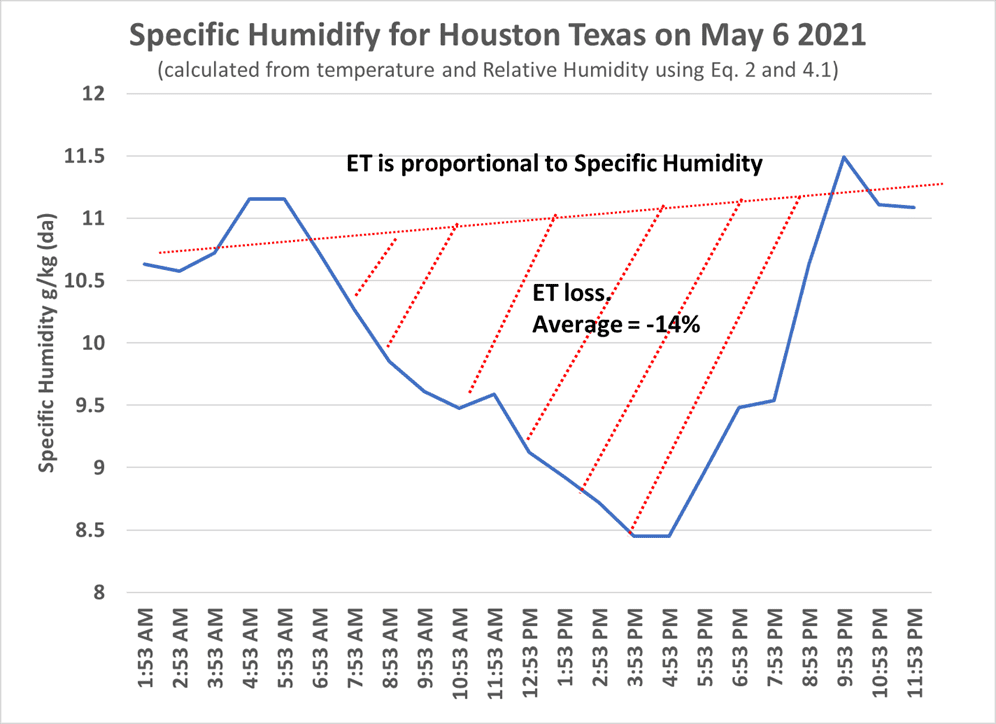
Figure 2 is an example of ET change in one day in Houston Tx showing a -14% reduction in SH in ½ day. This graph is obtained by using the hourly Temperature and Relative Humidity and calculating the Specific Humidity from Eqs 2 and 4.1. This lower ET air produces a plume, if the plume is the same size as Houston, then the daily ET is -7% (the plume is there for half a day) of the -14%. If the plume is 4 time the area of Houston the daily ET is 14*4*1/2 or -28%. The daily weather data does not tell us how big the plume is. Figure 1 is only one example to daily ET change. When it is raining or overcast the ET change is near 0% with no plume. If the parking lots and roads are wet when the sun comes out, the ET is positive. Daily plots of ET change in UHI’s can go as low as -40% to -50%. In a U. of Colorado paper [8] a lab experiment showed a 20-35% decrease in ET. Fu [15] and Zheng [16] show other examples of ET change in cities and forest to crop land in the -20% range. There is no consensus on what the global ET change is on the sum total of all the Earth’s Special Parcels. A range of 0 to -25% on the Special Parcel in this model is possible and will be tested.
Some of the latest papers on ET modeling and calculation are by Rigden [24] and Yan (25)
With out data on what total ET of all the Earth’s Special Parcels is, ET (SH) reduction in the Special Parcel is a Model variable.
2. Model Variable: The Plume
No measurement of plume size could be found. A model of plume size for Chicago by Cosgrove & Max Berkelhammer, (27), calculates a plume of 2 to 3 times the area of the city. Plume size should be a function of time the sun is out, time of the year, relative humidity of the air and the albedo of the surface. The bigger the density difference between the rising air and surrounding air the bigger the plume. With out data the Plume size is a variable in the Model
3. Model Variable: Size of the Special Parcel
The Special Parce is only land changes that cause the ET of that parcel to decrease. Examples are: a city, forest to crop, forest to pasture, reduction of flooded land, draining of marsh land, post forest fires, or mining. The model lumps all these types of land changes into one Special Parcel of land. The purpose of this model is to show how the fundamental variables of the Special Parcel land can change the global temperature. The sum total of all the Special Parcels is not an agreed to number.
For global cooing the Special Parcel may be different like new forest or new cooling towers, etc that put water into the air. Adding water to the air may reduce plume size due the lower density difference.
IV. Source of Physical Properties Equations
Six atmospheric variables are linked by Clausius- Clapeyron related Psychometric chart equations. With the use of these equations one can pick any 2 of the 6 variables and calculate the others. This Model uses this flexibility to transition from one step to the next step in the Model. The 6 atmospheric variables are: Temperature (T), Specific Humidify (SH), Relative Humidity (RH), Enthalpy (En), Dew Point (Td), Saturation Temperature, (Ts). (Specific Humidity, SH, is also known as Absolut Humidity or Humidity Ratio or Mixing Ratio). The preferred arrangement of these equation is shown in the Model’s derivation. The equations are Eq 2, 3, 4, 5, 6 and 9 (in Model Derivation)
The source of the equations is mainly from Vaisala Oyj [14] who has the simplest versions of the common equations. Similar equations can be found at [11], [12], and [13]
V. The Model’s basic data
Any model needs to fit the observed data. Data from NOAA [18] and HadISDH [6] were both candidates for the model’s derivation. The HadISDH [6] data were used because some of the NOAA southern hemisphere data had a very low R^2 vs time. The HadISDH [6] data were boiled down to 3 fundamental relationships plus the Climate Explorer CC data [5], Table 1 and Figure 6.
| Least squares fit vs year for HadISDH data 1975 to 2020 | |||
| observation | Eq vs year (x) | ||
| CC | y = -0.0753x + 212.77 | R² = 0.6486 | |
| Temp | y = 0.0209x – 27.297 | R² = 0.8799 | |
| SH | y = 0.0085x – 9.1539 | R² = 0.7568 | |
| RH | y = -0.0148x + 105.99 | R² = 0.4718 | |
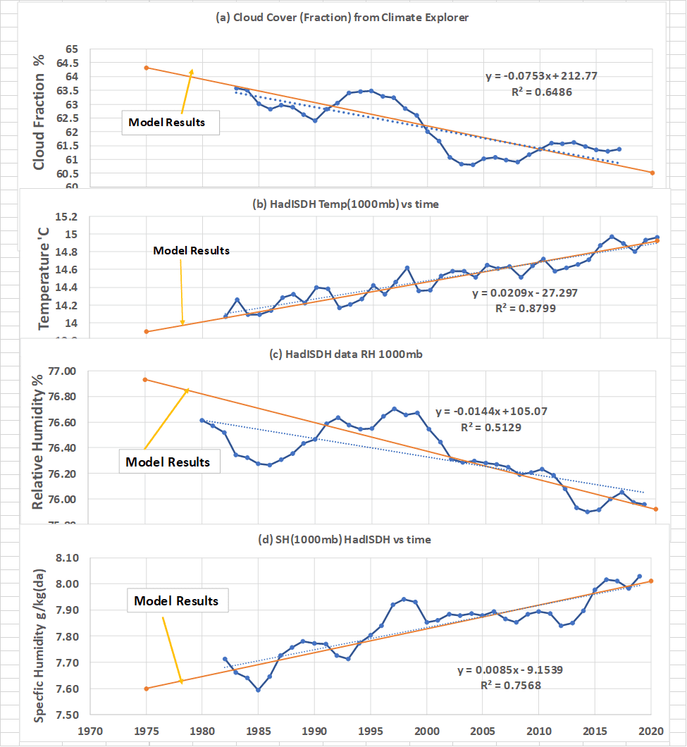
Table 1 basic data
To check the accuracy of the equations used in the Model four years were picked to compare calculation of the atmospheric variables to an on-line calculator [4] and this paper’s model’s equations. Table 2 shows the calculated Temp, RH, and SH for the selected 4 years with the equations in Table 1. The SH calculated vs Data error is shown to be good. The calculated by an on-line calculator [4] and this model are shown in Table 3.
| Basic DATA | |||||
| year | CC* | temp** | RH** | SH** | SH Calc-Data error |
| % | °C | % | g/kg(da) | ||
| 1975 | 64.05 | 13.981 | 76.76 | 7.6336 | 0.15% |
| 1982 | 63.53 | 14.127 | 76.66 | 7.6931 | 0.23% |
| 2011 | 61.34 | 14.733 | 76.23 | 7.9396 | 0.45% |
| 2020 | 60.66 | 14.921 | 76.09 | 8.0161 | 0.54% |
* Cloud Cover Data from Climate Explorer [5]
** Average yearly least squares fit of HadISDH [6] data
Table 2 basic data for four years and the error.
Comparison of on-line calculation vs this model’s calculations.
Table 3 On-line data from [4] vs result of this models calculated atmospheric variables using Equations 2, 3, 4, 5, and 6 (in Model Derivation).
Conclusions from Tables 1, 2, and 3 is Eq 2 thru 6 are ok to use in the Model.
VI. Special Correlations used by the Model
The following three relationships are used in the Model along with the atmospheric equations 2, 3, 4, 5, and 6 (in Model Derivation).
- Clouds vs |T-Td|
Cloud Cover has long been difficult to predict, see Walcek [22]. The variable chosen to predict probability of Cloud Cover (fraction) is the difference between the measure temperature (T) and the calculated Dew point temperature (Td), |T – Td|. (Figure 3.1 shows how |T – Td| changes on a psychrometric chart.)
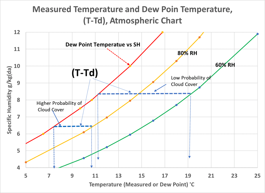
The Td value was obtained from HadISDH [6] data from average T and SH reported values using Equations 2 and 5. The Figure 3 correlation is a little better than the conventional relative humidity correlation.
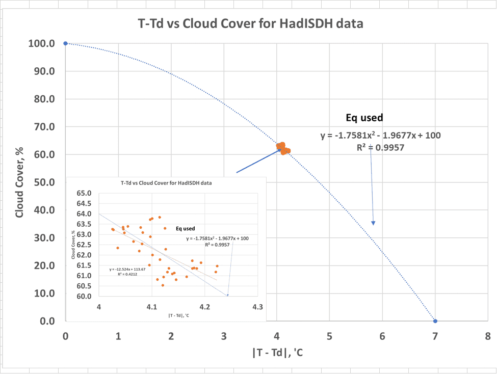
Figure 3 shows the HadISDH [6] data scatter plot with the linear least squares line (the insert plot in Figure 3). The correlation is improved by adding two common sense points: 100% cloud cover at 0 |T-Td| and 0 cloud cover at 7 |T-Td| (50-0% relative humidity = no clouds). The correlation then becomes a quadric. This quadric equation is used at each iteration of the model. The inserted graph in Fique 3 shows the used correlation goes through the scatter plot points. (The real cloud cover vs |T-Td| is probably more complex than Figure 3)
- Enthalpy and Cloud Cover
It is logical that changing cloud cover changes the atmosphere’s enthalpy. (somewhat related to W/m^2 as the earth’s albedo changes as cloud cover changes) The total enthalpy gain from less clouds goes to heat the oceans, add water to the atmosphere (increase SH), and heat the air. Figure 4 shows the correlation of cloud cover to Enthalpy for HadISDH [6] data using Equation 6 ) (in Model derivation) and the average annual T and SH.
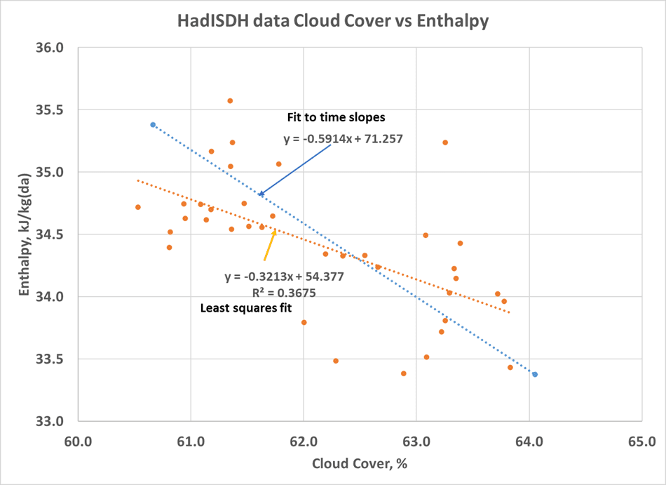
Figure 4’s R^2 not very good. Enthalpy vs cloud cover should be linear and Figure 4 give a range of values to try in the Model. The poor R^2 is due to the poor R^2 in the Cloud Cover vs time data. For comparison a line representing the slopes of the Enthalpy vs time and Cloud Cover vs time is also shown with a slope of -0.59 [(Enthalpy/time)/(Cloud Cover/time)]. The Model’s best fit to the data was -0.55 Enthalpy/Cloud Cover.
- Enthalpy and Specific Humidity
This relationship is needed to adjust the specific humidity for a Model’s iteration of new enthalpy. This relation is essentially Eq 6 (in Model Derivation). The Model lets Eq 6 calculate the Temperature. Figure 5 shows the correlation used in the Model.
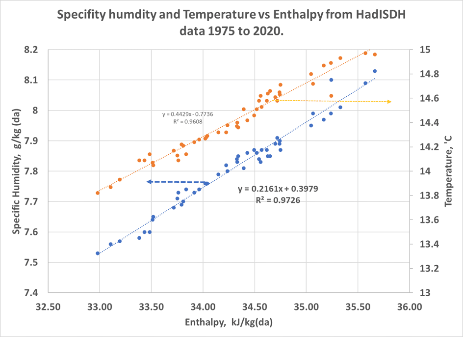
The Model could have gone from cloud cover to SH except the Enthalpy value was needed to calculate the T at each iteration.
VII. Model Results
- General Model Observations
The Model is a good match to observed 1975 to 2020 data of Cloud Reduction, temperature increase, Specific Humidity increase, and Relative Humidity decrease, see Figure 6. This match does not mean this Model is proof that ET reduction on Special Parcel is the cause of Global Warming from 1975 to 2020. A proof would require data that showed what the sum of all the Special Parcel variables really are, not an easy task. The Model, Figure 7 and Table 6, shows the many possible combinations.
A discovery from the Model is that the changes in the earths land mass ET (SH) will change the Earth’s temperature and the total ET (SH) of the earth in the opposite direction: A decrease in Earth’s land ET (SH) will result in an increase in global ET (SH) and temperature, or an increase in Earth’s land ET (SH) will result in a decrease in global ET (SH) and temperature. This suggest, in theory, that the Earth’s temperature can be controlled by manipulating the Earth’s land ET (SH). In theory, this control could offset any greenhouse gas, albedo, or volcano issue. If the Earth’s temperature could be controlled, what would be the best temperature?
The ET (SH) change of the Special Parcel has a -1 : +10 amplification factor on global ET (SH) change; that is, a -1% change (as a % of total global ET (SH)) will result in a +10% change in global ET (SH). This unusual amplification is due to the high negative sensitivity of cloud formation to |T – Td| in Figure 3 and the fact that most of the earth is cover by water where any change is cloud cover will increase water evaporation 5x more over all the water vs all the land (27), this is imperially included in the Model by Figure 4 where Cloud cover is related to observed enthalpy.
2. Sensitivity to the Special Correlations.
Table 4 shows the results of a sensitivity test on the three Special Correlation used in the model:
- Cloud Cover vs |T – Td|
Could not find a correlation in the literature for this special relationship. The use of anchors at [100% CC and zero |T- Td|] and [zero CC and |T-Td| ] at each end of the observed data seems to give a sensible curvature to the relationship and prevent out of bounds values in the convergence iterations. Several zero cloud cover intercepts were tested (an example of 3 are show in Table 4). The best fit to cloud cover was an |T-Td| zero intercept of 7 ‘C.
b. SH vs Enthalpy
Cannot be changed much outside of Figure 5 slope. Figure 5 good correlation is related to Eq (6).
- Enthalpy and Cloud Change
This relationship is one of the biggest unknows in the model. The use of -0.55 Enthalpy change per Cloud Cover change seems to give the best fit to the observed Cloud Cover. This fit of -0.55 En/CC is very close to the slopes of the En vs time divided by SH vs time line. This relationship is needed for the model because it estimates how much of the increase in energy (from Cloud Cover decrease) go to the atmosphere increase in SH vs other palaces (like the oceans).
Table 4. Sensitivity to Special Correlation.
With the Special correlation fixed the model can be used to explore the Special Parcel variables. As Table 5 shows the Model is sensitive to all three variables, ET change, Area, and Plume size. This temperature sensitivity is only calculated from the fixed special correlations and the atmospheric equations 2,3,4,5, and 6. The atmospheric equations are changing the GW results!
Table 5. Model results from changing the three Special Parcel variables.
In Table 5 the observed starting conditions of 1975 and end conditions of 2020 are shown. (The 1975 entry for Special Parcel area and plume size is canceled out by the 0.0 change in ET.) The 2020 labeled conditions are not unique there are lots of ways to get to the 2020 observed results as Table 6 shows.
Table 6. Some of the many ways the Special Parcel area, plume size, and ET change can be changed and get the same 2020 results.
VIII. Probable range of Special Parcel variables
The emphasis of this paper is the development of a model. Discussion of what the real range of Special Parcel values can be found in the reference list of this author’s other paper’s [1], [2], and [3]. The following range of possibility is suggested.
- ET decrease in Special Parcels: a range on 0 to -25% ET change (change during day time).
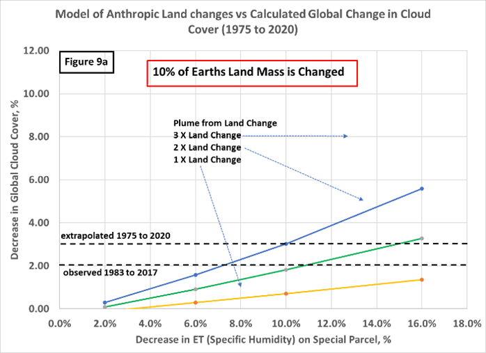
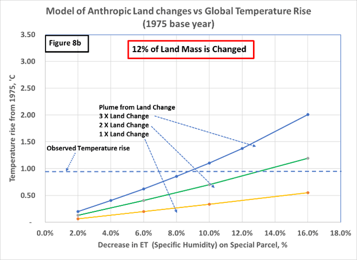
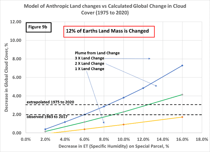
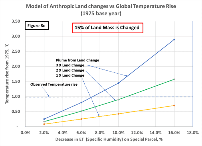
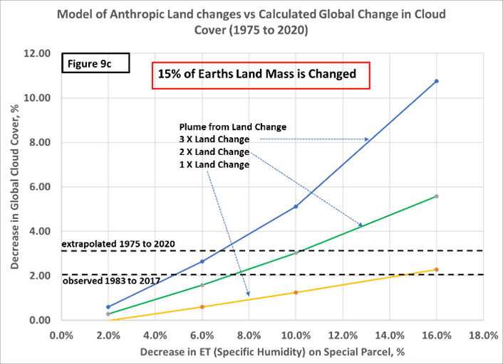
- Special Parcel Area: 10% to 15% of the land mass of the Earth
- Plume size from the Special Parcel: 1 to 6 times the area of the Special Parcel area.
Figure 7 show a graphical profile of the possible fits of Special Parcel variables to the observed 1975 to 2020 temperature increase.
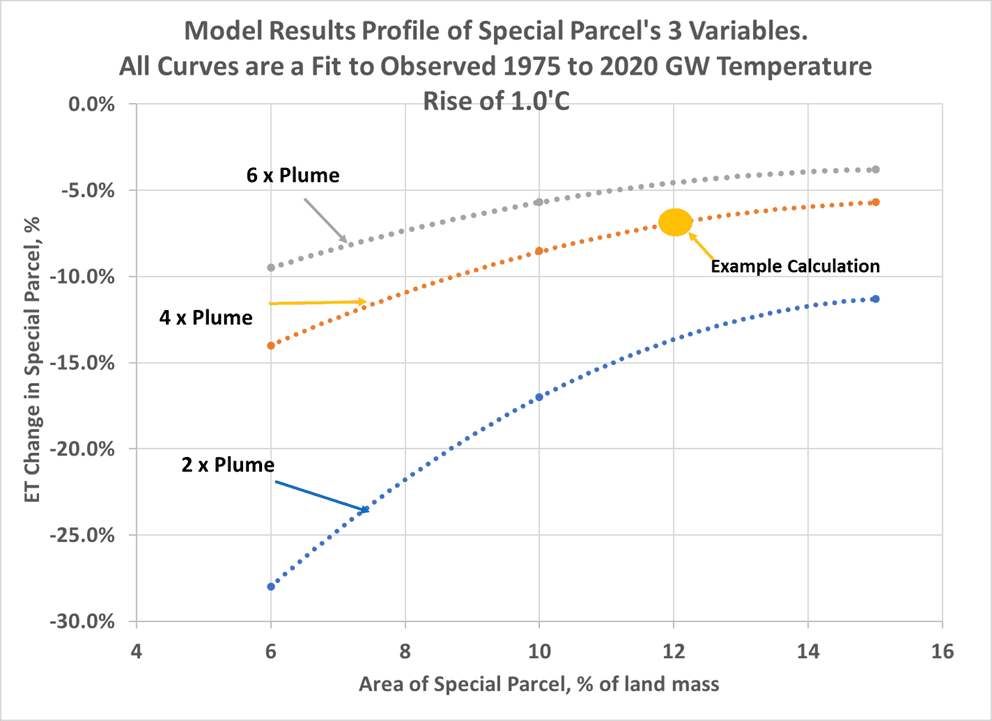

IX. Global Cooling
The Model is reversable. If the ET on the Special Parcel is increased the temperature decreases, Figure 10. To reduce global temperature from 2020 to 1975 levels an increase of 12% ET (SH)/year on the Special Parcel (12% of land mass and plume factor of 2x). This +12% ET on the Special Parcel is equivalent to 0.4%/year of the Earth’s total ET, Table 6 shows the derivation.
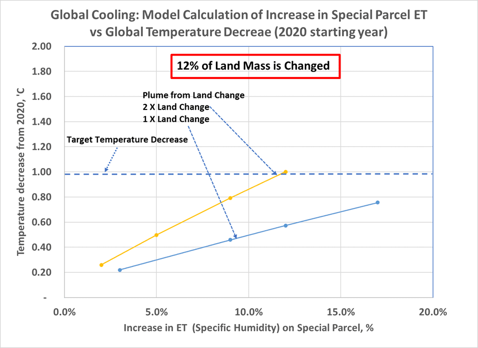
Trees are the natural way to put water back into the atmosphere. Trees with their many leaves and deep roots can put a lot of water into the atmosphere if enough water is available in the soil. (A tree sounded by concrete is not as efficient as a tree in a rainforest at getting water back into the atmosphere.)
One example of how to add water to the atmosphere is power plant cooling towers. Not all power plants have cooling towers some use river or ocean water to cool the turban’s spent steam. What if all the Earth’s electricity was generated with power plants with cooling towers that put water back into the atmosphere, that water would be 40% to the total needed to return to 1975 temperatures (not a serious proposal just an example), see table 6.
One more example; water misters on heat pump exhaust fans and hot pavement.
Be creative.
Table 6 Global Cooling calculations.
X. Predicting Possible Future Temperature Rise
The size of the Special Parcel is expected to increase as the population of the Earth increases. The ET and Plume associated with this population increase is expected to remain relatively constant. Assuming the same rate of increase in population from 1975 to 2020 as 2020 to 2065 the Model calculates a temperature rise of 2.6 ‘C, see Figure 11.
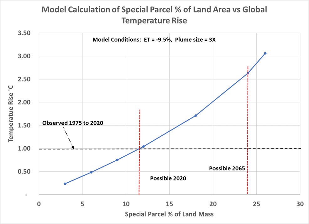
Note the upward curvature of Figure 11 from the non-linear Figure 3. This Figure 3’s quadratic function causes the Model to fail above 28% Special Parcel % of land mass, suggesting the Model need a more complex Figure 3 function for extreme values of the Model’s variables.
XI. Conclusions
The Model suggest that ET changes on the Earth’s land surface controls the Cloud Cover which in turn control the Earth’s temperature. This mathematical observation is probably not new to climatologist, who model ET seasonal and Northern vs Sothern hemisphere difference over a year. The change in anthropic land use over years may be new and this Model show one way Cloud change can happen.
This Model of GW from a Special Parcel’s ET change is fit to the Earth’s 1975 to 2020 observed temperature rise. It fits the observed profile of Specific Humidity rise, and Relative Humidity decrease. This Model may be a unique calculation of local ET change and GW. This Model is a proof that a local change in ET is related to an increase in GW, but is not a proof that it does. Modeling is a good first step in a proof. A proof would require data on what the real size of this Special Parcel is and what is the average ET drop and Plume size.
This Model was created to encourage scientist to collect the information necessary to determine the Earth’s ET change over time, the area of “special parcels” and plume size. This Model shows that this data is necessary for our complete understanding of Climate Change.
XII. Appendix
The Model Derivation
Figure 1 shows a diagram of the Model. The basis of the Model is the Earth’s natural water cycle calculated from standard atmospheric Clausius–Clapeyron related Psychometrics chart equations at each step. The Model’s steps are coupled with the three observed correlations above: 1) “Temperature – Dew Point Temperature” (T-Td) vs Cloud Cover, CC, (Fraction), 2) Enthalpy, En, vs Cloud Cover, CC, and 3) SH vs Enthalpy. These three correlations are logical relationships but due to the uncertainty in Cloud Cover have a high range of uncertainty – this will be explored. The Cloud Cover (Fraction) uncertainty is most likely due to the transition between no clouds and thin clouds (see paper [3] for more details). The values of these three correlations best fitting the observed cloud cover change will be used in the final Model that calculates response to Special Parcel variables.
The steps of the Model start with the description of a Special Parcel of land that has be changed in a way that the ET of that parcel has decreased (or increase for Global Cooling).
This Derivation is presented in a format that can be entered into an Excel type program and test the Model for yourself.
Step 1
The starting year of the Model is chosen. The example uses 1975. The following data for that year is determined from historical data, see table 1 for examples. The Model’s starting variables are Specific Humidity (SH(1)), Temperature (T(1)), and Cloud Cover (CC(1)). From these variables the dew point Temperature, (Td(1)), Relative Humidity (RH(1)), and Enthalpy (En(1)) can be calculated. The model relies on accurate vapor pressure for water at saturation, Pws, and at desired conditions, Pw. More complex vapor pressure models are available for wider temperature and pressure ranges. The ones used for this model fits the range of Earth’s atmospheric temperatures.
Water’s saturation, Pws, pressure is from Vaisala Oyj [14]:
Pws(1) = 6.116441*10^((T(1)*7.591386/(240.7263+T(1)))) hPa Eq 2
Waters vapor, Pw, pressure is from Vaisala Oyj [14]:
Pw(1) = SH(1)*1013/(621.9907+SH(1)) hPa Eq 3
The relative humidity, RH, is defined as [14]:
RH(1) = Pw/Pws*100 % Eq 4
SH = Pws*RH/100 (used for Figure 2) Eq 4.1
The dew point temperature, Td, is calculated [14]:
Td(1) = 240.7263/(7.591386/LOG(Pw(1)/6.11644,10)-1) ‘C Eq 5
And the Enthalpy, En, of the starting condition is determined by Vaisala Oyj [14]:
En(1)= T(1)*(1.01+0.00189*SH(1))+2.5*SH(1) kJ/kg (da) Eq 6
The starting |T-Td|(1) is calculated.
These conditions are for the entire Earth’s atmosphere at ground level including the Special Parcel at starting conditions.
Step 1 example for 1975
| CC | SH | Temp | RH | Enthalpy | Dew Temp. | Pws | Pw |
| % | g/kg(d.a) | ‘C | % | kJ/kg(d.a) | ‘C | hPa | hPa |
| 64.05 | 7.63 | 13.98 | 76.93 | 33.41 | 10.00 | 15.97 | 12.28 |
|T – Td| (1) = 13.98 – 10.00 = 3.98’C Eq 7
Step 2.
For the Special Parcel a decrease in ET is chosen (for the end year). Literature suggests a value between 0 and -30%. The example will use -7% ET change. Since ET is proportional to SH, a SH change for a -7% change in ET is -7%. The ET and SH proportionality is on an annual basis where the other variables (wind and updraft) should be relatively constant year to year.
SH(2) = (1+ET) * SH(1) g/kg(da) Eq 8
The enthalpy of the special parcel at starting conditions is the same as the whole Earth. The atmospheric conditions of the special parcel’s air can be calculated from the equations:
T(2)=(En(1)-2.5*SH(2)/(1.01+0.00189*SH(2)) Eq 9
Pws(2) = 6.116441*10^((T(2)*7.591386/(240.7263+T(2)))) repeat Eq 2
Pw(2) = SH(2)*1013/(621.9907+SH(2)) repeat Eq 3
RH(2) = Pw(2)/Pws(2)*100 repeat Eq 4
Td(2) = 240.7263/(7.591386/LOG(Pw(2)/6.11644,10)-1) repeat Eq 5
En(2) = En(1)
Example Step 2 Special Parcel properties at a -7.0% ET change:
| CC | SH | Temp | RH | Enthalpy | Dew Temp. | Pws | Pw |
| % | g/kg(d.a) | ‘C | % | kJ/kg(d.a) | ‘C | hPa | hPa |
| NA | 7.10 | 15.30 | 65.76 | 33.41 | 8.93 | 17.38 | 11.43 |
This air is hotter, lower RH, less dense than the surrounding air so it rises in a plume to the level of cumulus clouds. The size of this plume of air from the special parcel is:
PA = (1-EO) * SP * PF * DN, (% of the Earth) Eq 10
Where:
SP = Special Parcel Area, % of the Earth’s land mass
PF = Plume factor (how much bigger than the land is the plume) from the Special Parcel.
EO = Area of the Earth that is Oceans, (71%).
DN = Day – night factor. Fraction of the day the plume is generated. (0.5).
Example Step 2 Plume area calculation:
| SP | PF | EO | DN |
| % of Land | factor | % | fraction |
| 12.0 | 4 | 71 | 0.5 |
PA = 6.96% of the Earth
Step 3
The picture in mind at this step is: a vapor cloud rising from a cooling tower. When it reaches cumulus cloud level a plume forms at a constant level and goes downwind. At some distance the plume starts to disappear. With this Special parcel plume, we can’t see it.
This plume of air from the Special Parcel (step 2) mixes with the atmospheric air in step 1 with the energy balance equations:
SH(3) = SH(1) * (1-PA) + SH(2) * PA Eq 11
T(3) = T(1) * (1-PA) + T(2) * PA Eq 12
This mixed air now has a lower relative humidity and higher temperature that can thin or prevent cloud formation.
Example Step 3 air properties are now after -7% ET change and mixing:
| CC | SH | Temp | RH | Enthalpy | Dew Temp. | Pws | Pw |
| % | g/kg(d.a) | ‘C | % | kJ/kg(d.a) | ‘C | hPa | hPa |
| 61.64 | 7.60 | 14.07 | 76.10 | 33.41 | 9.93 | 16.06 | 12.22 |
Note: In reality as this air rises the atmospheric pressure decreases and the real temperature of this air decreases as the laps rate predicts. Since all the special correlations are biased on ground level data the mixing in this step will be treated as ground level, since no higher altitude atmospheric equations are used. Cloud Cover is related to ground level data. (This model could be improved with a mixture of ground level and cumulus cloud level correlations).
Step 4
|T-Td| is calculated:
|T – Td|(3)= 4.11’C
Using the Figure 3 correlation of |T-Td| we can get an initial estimate of Cloud Cover CC(3).
CC(3)= -1.7581 * |T-Td|(3)^2 – 1.9677*|T-Td|(3) + 100 Eq 13
and Cloud Cover change
CCc(3) = CC(3)-CC(1) Eq 14
The reduction in cloud cover lets in more sun to the Earth thus increasing the Enthalpy. From Figure 4 the correlation of Cloud Cover change, CCc(3) can be related to Enthalpy, En(3)
En(3) = CCc(3) * -.55 + En(2) Eq 15
The Cloud Cover decrease (or cloud thinning) lets more sun in to the earth surface, evaporating water mostly in the oceans (E part of ET) and a slight increase in the T part of ET. The SH increase is correlated to the Enthalpy as show in Figure 5. An increase in SH(3) due to the increase in Enthalpy can now be calculated
SH(4) = (En(3) -En(2)) * 0.216 + SH(3) Eq 16
Assume Enthalpy in step 3 is the same at the Enthalpy in Step 4 (part of an iteration process).
En(4) = En(3)
Calculate T(4) with Eq 9 using SH(4) and En(4).
With SH(4) and T(4) now known, the other atmospheric properties can now be calculated by repeating Equation 2, 3, 4, and 5. To get Pws(4), Pw(4), RH(4), and Td(4).
Example for Step 4
| CC | SH | Temp | RH | Enthalpy | Dew Temp. | Pws | Pw |
| % | g/kg(d.a) | ‘C | % | kJ/kg(d.a) | ‘C | hPa | hPa |
| 60.96 | 7.88 | 14.66 | 75.99 | 34.73 | 10.48 | 16.68 | 12.68 |
Repeat all the in step 4 with new |T-Td|(5) from above. Then new CCc(5) with Eqs 13 and 14. Then new En(5) with Eq 15. Then new SH(5) with Eq 16. Follow up with the other atmospheric properties by repeating Equation 2, 3, 4, and 5. To get Pws(5), Pw(5), RH(5), and Td(5).
Note in all iterations SH(3) in Eq 16 and En(2) in Eq 15 are held constant. This is because they are the change from the Special Parcel ET change the remaining changes are from the Cloud Cover change.
This will take about 4-6 iterations.
Example after 6 iterations at -7.0% change in ET in Special Parcel:
| CC | SH | Temp | RH | Enthalpy | Dew Temp. | Pws | Pw |
| % | g/kg(d.a) | ‘C | % | kJ/kg(d.a) | ‘C | hPa | hPa |
| 60.57 | 8.01 | 14.92 | 75.92 | 35.32 | 10.71 | 16.97 | 12.88 |
Bibliography
- Climate Explorer: Select a monthly field (knmi.nl) go to “Cloud Cover” click “EUMETSAT CM-SAF 0.25° cloud fraction” click “select field” at top of page on next page enter latitude (-90 to 90) and longitude (-180 to 180) for whole earth.
- . Loeb,Gregory C. Johnson,Tyler J. Thorsen,John M. Lyman,Fred G. Rose,Seiji Kato web link Satellite and Ocean Data Reveal Marked Increase in Earth’s Heating Rate – Loeb – 2021 – Geophysical Research Letters – Wiley Online Library
- Stack Exchange Network web link thermodynamics – Equations instead of psychrometric charts – Physics Stack Exchange
- Equations for the Determination of Humidity From Dewpoint and Psychrometric Data (nasa.gov)
- Vaisala Oyj web link Humidity_Conversion_Formulas_B210973EN-F (hatchability.com)
- Long‐term change of total cloud cover and its possible reason over South China during 1960–2012 – Fu – 2019 – Atmospheric Science Letters – Wiley Online Library
- Michael Jonas web link Clouds Haven’t Behaved the Way the IPCC Or the Models Say – Watts Up With That?