by Bruce Peachey and Nobuo Maeda
Contemporary climate models only include the impact of water vapor as positive feedback on warming; the impact of direct anthropogenic emissions of water vapor has not been seriously considered.
Background
Recent climate change and increasingly scarce fresh water resources are two major environmental issues facing humanity. Water vapor is the most abundant greenhouse gas. Contemporary climate models only include the impact of water vapor as positive feedback on warming; the impact of direct anthropogenic emissions of water vapor has not been seriously considered.
Our recent publication used the NCEP/NCAR reanalysis data set to examine whether the Clausius−Clapeyron equation can form a basis for such positive feedback commonly assumed in the contemporary climate models [1]. We found that: (1) qualitatively, the log-linear nature of the Clausius−Clapeyron equation [(ln Pv) vs (1/T)] demonstrates a significant level of consistency when averaged over expansive regions like specific latitude zones around the globe; (2) this consistency does not extend to individual locations where a plot of (ln Pv) vs (1/T) becomes nonlinear, indicating substantial undersaturation that varies with time; (3) quantitatively, the discrepancies between the locally observed and the expected values of the slopes of (ln Pv) vs (1/T) are wide-ranging; and (4) the absolute amount of water vapor has increased substantially above the population centers and the agricultural areas in the Northern Hemisphere between 1960 and 2020, but not in the Southern Hemisphere where the surface area of the oceans is much greater. These findings suggest that direct anthropogenic emissions of water vapor are an important driver that influences the local water vapor content.
Our paper concluded that the use of the Clausius–Clapeyron equation as a basis for calculating the positive water vapor feedback appears to be on shaky ground [1]. Since the discrepancies between the observed and the expected values of the slopes of (ln Pv) vs (1/T) were wide-ranging [1], it remains unclear if the amount of atmospheric water vapor will truly increase by as much as 6 to 7% in response to every 1 °C of warming, as commonly assumed.
In the present contribution, we highlight: (1) the role of humans in the global water cycle and impacts on climate change, (2) the regional nature of many aspects of “global” warming, (3) propose that future research effort should be directed toward obtaining the relevant data as a matter of urgency.
Water cycle
Human activities indeed have been impacting climate but most of the key factors are related to water, as opposed to CO2 [2-6]. Atmospheric water vapor increase in the Northern Hemisphere has been by several percent per decade. In contrast, there has been little change in the Southern Hemisphere. Unlike water, CO2 is in a single phase and largely uniformly distributed in the atmosphere. Thus, if CO2 were the cause of the current climate change, and if the ocean is the source of the water vapor that is supposed to increase by about 6 to 7% in response to every 1 °C of warming caused by the non-aqueous greenhouse gases, then the Southern Hemisphere should have observed more of the consequences than the Northern Hemisphere due to its much larger surface area of the oceans. To the contrary, a 2% average increase in precipitation, that amounts to an average of about 2 Tt/year over the last century, has been observed in the Northern Hemisphere land precipitation, while no such increase was observed in the Southern Hemisphere land precipitation [7]. This increase in the Northern Hemisphere land precipitation has been accompanied by an estimated 2 to 4% increase in the frequency of heavy precipitation events in the last 50 years, again in the Northern Hemisphere but not in the Southern Hemisphere.
Water is being consumed by humans at an increasing rate, predominantly in the Northern Hemisphere, at least by 3 to 4 Tt/year (excluding some sources such as reservoir evaporation). This increasing water consumption has been accompanied by reductions in the return flows of the fresh water to the oceans from the rivers in regions with intensive irrigation & industry, again predominantly in the Northern Hemisphere. Other major contributors identified by the IPCC are water emissions and land use. Calls for the comprehensive integration of substantial changes in the hydrological cycle into global climate models are not new [8, 9], but have received limited support, and consequently these causes have generally been ignored and not incorporated into the contemporary climate models to date.
Natural land water flux is based on water vapour coming on to land areas from the ocean, water falling as precipitation with some being re-evaporated from the landscape with the remaining flow, of about 40 Tt/yr, flowing back into the ocean to balance the flow of water vapour from the ocean. Ocean water vapor flux is 6 times larger than the land water vapor flux, even though the global water surface area is only about 3 times larger than the land area [2]. This is because: (1) the ocean surface is darker and hence absorbs more solar energy and (2) the ocean surface is always wet, which enhances mass transfer compared to the land surface, which sometimes is wet and sometimes is dry. At any one time, the atmosphere contains about 13 Tt of water, which contributes most of the greenhouse effect, and a given water molecule on average only spends about 10 days in the atmosphere each time it goes through the cycle [10].
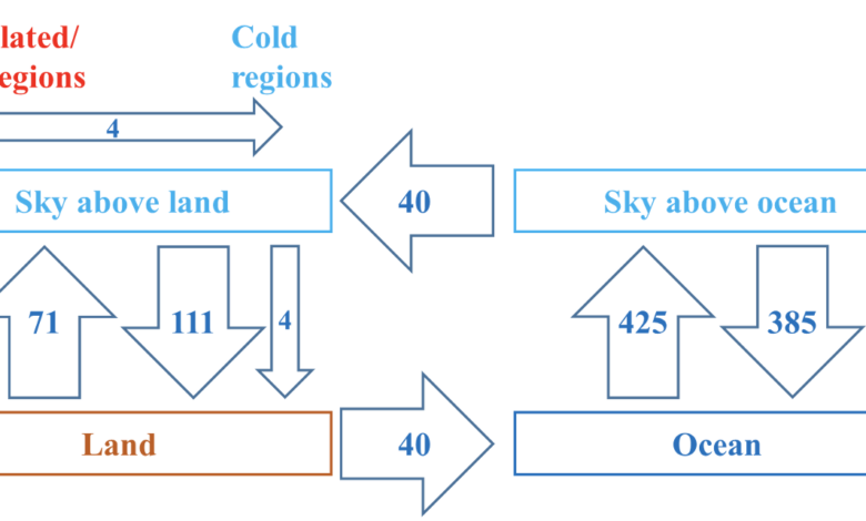
Global water budgets are found in many publications on water availability and show some variations in numbers used, but are within a reasonable range, and generally agree with each other. For this analysis, we show schematically a global water budget in Figure 1, which uses the numbers from “Global Warming – The Complete Briefing” by Houghton [11]. Here we assume that the total amount of water in the atmosphere does not change materially in a short time span of a year (after all seasons in a year), notwithstanding the fact that warming leads to increased water vapor content.
More recent literature (https://www2.whoi.edu/site/globalwatercycle/) provides slightly different numbers of (after converting the unit of m3/s to Tt/yr) 41 instead of 40 for the horizontal land to the ocean water flux, 69 instead of 71 for the upward land to land atmospheric water flux in Figure 1, 110 instead of 111 for the downward land atmosphere to land water flux, 426 instead of 425 for the upward ocean to oceanic atmosphere water flux and the same 385 for the downward oceanic atmosphere to ocean water flux, which provides the readers with an idea of the amount of variations involved. Our conclusions will remain unaltered regardless of which version of numbers we use.

Figure 1 Global conservation of water masses adapted from [2]. The numbers show the movement of water masses in tera tons per year. This is the base case before the recent warming became an issue.
The numbers in Figure 1 show the movements of water in tera tons (1 Tt = 1012 t = 1015 kg) per year before the recent warming. The inflows and the outflows of water must be balanced at each reservoir of “land”, “ocean”, “sky above land” and “sky above ocean”, to satisfy the conservation of mass. These four entities can, but do not need to, be geometrically continuous.
Water withdrawal and water use data is available from a number of sources and studies. Most estimates put human water withdrawals in the range of 4 to 5 Tt/yr worldwide, with over 60% of that going to irrigation, 20 to 30% to industrial cooling and the remainder for domestic use. For example, the IPCC’s estimate of anthropogenic water withdrawals that are reducing ocean discharge flows in rivers such as the Nile, Colorado, Yellow, Rio Grande, and other rivers that are heavily used for irrigation places the reduction in the return flows to the ocean (the 40 Tt from “land” to “ocean”) is around 10%, or 4 Tt/yr [7, 12]. Houghton reports “in the United States, for the Missouri river basin it is 30%, for the Rio Grande it is 64%, and for the lower Colorado 96%. Almost none of the water in the Colorado river reaches the sea” [11]. In short, the water consumption on such river systems as a percentage of the total discharge can be substantial. More recently, the latest 2021 IPCC Climate Change report reported the magnitude of the impacts humans have had on water cycle on land in that: “Direct redistribution of water by human activities for domestic, agricultural and industrial use of about 24,000 km3/year is equivalent to half the global river discharge or double the global groundwater recharge each year” [13]. Therefore this 24 Tt/yr is ~60% of the total estimated return flow of 40 Tt/yr to the oceans.
Unfortunately, these reports do not provide an explanation as to where the water goes after it has been withdrawn or redistributed. Consequently, what is less clear is the actual amount of evaporation of water to the atmosphere. For irrigation withdrawals, most of the water is evaporated during irrigation or from the field after irrigation, whereas for most domestic water withdrawals the water may be returned to the source or another water body as sewage. The main industrial water use is for cooling thermal plants, however, the relationship between withdrawals and evaporation loss of water varies greatly, depending on the cooling process used (i.e. evaporative cooling on-site or return of hot water to a large body of water). Some data sources breakdown water volumes by use, by water basin, or by country with accuracy varying depending on what is being reported, consistency in the reporting, measuring methodologies, and the rigour applied to the data collection process [11, 14-21]. Often these estimates do not include other water losses, where the water transfer is unintentional or unmeasured, such as losses to groundwater reservoirs, or evaporation from hydroelectric or irrigation reservoirs, they may also not contain withdrawals of groundwater from aquifers which have greatly increased in recent years [22].
A major challenge for a contemporary climate model is: How to generate a 5% increase in land precipitation in Northern hemispheric land areas, which has been reported to occur in the IPCC reports [7, 12], but not in Southern hemispheric land areas?
Since the Northern Hemisphere contains 67.3% of the Earth’s land, if we neglect the Southern hemispheric land precipitation increases for simplicity, the increased Northern hemispheric land precipitation by 5% would result in about 3.4% increase in global land precipitation. Such 3.4% increase of the 111 Tt downward water flux over the entire landmass equates to about 4 Tt extra downward water flux. Under the contemporary non-aqueous greenhouse gas-driven global warming paradigm, this extra 4 Tt would have to come from the oceans through a 10% (of the 40 Tt) increase in the water vapor content of air crossing onto land masses from the oceans. Now, one cannot realistically assume that 100 % of this extra water vapor generated from the ocean surface will exclusively flow to the land: the majority should precipitate back onto the ocean.
For simplicity, here we assume that the same proportion of the water vapor generated as that shown in Figure 1 would partition into the land and to the ocean downward fluxes. Then, to generate the 4 Tt increase in the water vapor content on the landmass, both the upward and the downward water fluxes over the entire ocean surface must also increase by 10% over historic levels. Then, the resulting global water balance (without considering the Northern vs Southern hemispheric water partitions) would look something like what we schematically draw in Figure 2.

Figure 2 Global conservation of water masses that corresponds to the settings assumed by the contemporary climate models. The numbers show the movement of water masses in tera tons per year. Non-aqueous greenhouse gases initiate a positive feedback in which the initial warming leads to increased evaporation from the oceans of 42 tera tons per year. 38 of the incremental 42 tera tons would directly precipitate back onto the ocean and 4 out of the 42 tera tons would transport to over a land area before precipitating. The 4 tera tons of the excess water that has precipitated on the land would need to flow back to the ocean to close the water cycle, which is contrary to the observations.
The purported change of water from the oceans to the land areas to account for increased land precipitation would generate a significant (+10%) increase in total water outflow off continental land masses (the return flow of about 4 tera tons to compensate for the excess water evaporated from the ocean as a part of the purported positive feedback mechanism in the contemporary climate models), as shown in Figure 2, which is incidentally contrary to the observations that show dwindling outflows of major rivers around the globe [7, 12]. Nor does it explain how the only area showing incremental precipitation is the latitude band from 30 to 60 degrees North, with no significant change in the Southern Hemisphere.
The water mass balance (budget) above also has significant energy balance implications. To achieve the required 42 Tt/yr of incremental water evaporation off oceans would require a large amount of incremental solar energy being absorbed. We estimate that this would require on the order of 10 Zeta Joules/year being absorbed by the oceans (42 Tt/yr × 2260 kJ/kg) or a 10% increase in solar energy absorbed. Given that the average estimated incremental radiative forcing is ~ 2 W/m2 of the earth’s surface, it is much more realistic to assume that the incremental radiative forcing would proportionately partition so that the ocean to the oceanic atmosphere water flux would increase by ~ 2 [W/m2] / 300 [W/m2] × 425 [Tt/yr] = 2.8 Tt/yr, assuming the 300 W/m2 is the net average radiation absorbed by the earth and 425 Tt/yr being the upward water flux over the oceans (note our conclusion remains unaltered even if the correct number were 200 W/m2 or 400 W/m2 as the net average radiation absorbed by the earth). Then, about 10% (the same proportion as in Figure 2) of the 2.8 Tt/yr incremental water vapor, or 0.28 Tt/yr, would transfer to land areas while the rest would precipitate back to the ocean, which would be considerably less than the 4 Tt/yr incremental precipitation observed over land areas. In short, the scenario envisioned in Figure 2 is highly unrealistic.
Figure 2 is for the global water mass balance and hence does not account for any regional-scale details. From a regional water mass and energy conservation perspective, an intensified non-aqueous greenhouse gas effect resulting in global warming should have a much greater impact on climate in the Southern Hemisphere because its fraction of the ocean is far greater. Yet the IPCC climate data shows a definite bias towards precipitation from climate change being a predominantly Northern Hemisphere phenomenon, and the total precipitation over the Southern Hemispheric land masses has not increased [7, 12]. The contemporary climate model simulations show that most of the extra evaporation to originate in the Southern Hemisphere, so it leaves the question open as to how the water vapour purportedly generated in the Southern Hemispheric oceans preferentially crosses into the Northern Hemispheric land masses.
To the contrary, the areas of increased precipitation tend to be in cool wet Northern areas, fed by air masses from hot, dry or highly populated areas, with high anthropogenic water emissions, which are unassociated with “global” warming. The main region in the Southern Hemisphere, which shows a similar response to the Northern Hemisphere, is Patagonia in South America, which has an irrigation and energy intensive economy. Patagonia, through ocean and atmospheric circulation patterns, feeds water and energy to the Antarctic Peninsula, which is the only part of Antarctica to show any impact of “global” warming [23]. Since the latent heat of vaporization of water is large, one tonne of water vapour contains enough energy to melt 6.7 tonnes of ice or snow. An analysis should be undertaken as to the relationship between the water use in Patagonia and deterioration of ice masses on the Antarctic Peninsula.
Other regions in the Southern Hemisphere, such as New Zealand, the western coasts of Australia and Southern Africa, show little change in precipitation that they should have experienced with increased water evaporation from the oceans that is purported to occur under the non-aqueous greenhouse gas-driven, water vapor positive feedback amplified, paradigm. To the contrary, the South Island of New Zealand, with its high mountains and the Tasman Sea to the west and should have experienced substantially more precipitation, has not. In Australia, the coasts of Western Australia remain dry, and increased precipitation and extreme heavy rainfalls instead occur in Eastern Australia which is downwind of the water withdrawn from the Murray–Darling Basin for irrigation.
Since there is sufficient evidence / observations that support the idea that anthropogenic emissions are an important driver of recent warming [1], we now consider how the conservation of water masses might look like if anthropogenic emissions of water vapor were indeed the primary driver of the recent trend of climate warming. As noted above, wetter land surfaces and new vegetative cover after irrigation are darker than the dry surfaces before irrigation, and consequently absorb more sunlight. The concomitant incremental radiation energy absorbed through increasing the area of absorption by spreading water from lakes, rivers and underground aquifers over fields and rice paddies is still an incremental energy input, and must be released by the water during condensation (cloud formation) and precipitation in the Northern areas. Anthropogenic emissions of water vapor, which is predominantly emitted in the low to mid latitudes of the Northern Hemisphere (between 0 and 60°N), would move water and energy poleward to the Arctic through atmospheric circulation patterns.
The condensation of water vapor would release latent heat, cause melting of Northern and inland ice sheets, increase Northern cloud cover, and increase precipitation and severe weather events, wherever the water comes out. Such movements of water masses also explain the reported freshening trend in water flowing to the Arctic, Atlantic and Pacific, and the increasing salinity and temperature increases in tropical water masses, which are no longer receiving those cool fresh water returns from rivers. Figure 3 shows how the water balance might look like in this scenario. As was the case in Figures 1 and 2, Figure 3 is for the global scale description that does not include any granularity or geographical spread of each of land and ocean components.

Figure 3 Global conservation of water masses when the Anthropogenic Emissions of Water Vapor is assumed to drive the recent trend of climate warming and climate change. The numbers show the movement of water masses in tera tons per year. Here, extra 4 tera tons per year of water vapor would be generated from the land and virtually all of them precipitate back on the (colder parts of) the land.
As we did during the calculation of the water mass balance in Figure 2, since the Northern Hemisphere contains 67.3% of the Earth’s land, if we neglect the Southern Hemispheric land precipitation increases for simplicity, the increased Northern Hemispheric land precipitation by 5% would result in about 3.4% increase in global land precipitation. Such 3.4% increase in the 111 Tt downward water flux over the entire landmass equates to about 4 Tt extra downward water flux, which has been observed to be concentrated in the cold Northern Hemispheric landmass. Unlike in Figure 2, however, the extra 4 Tt does not come from the sky above ocean, but instead comes from the warm, dry and/or populated regions of the landmass.
On a regional basis, anthropogenic emissions of water vapor also better match the observations of reduced flows in highly utilized rivers and lakes in dry, heavily populated regions such as China, India, Pakistan and the southwestern United States, and the corresponding increases in rainfall in Northern temperate regions. Examples of regional–scale “unusual patterns” include: (1) weekly patterns of rainfall on the east coast of the United States showed that rainfall was 22% higher on Saturdays than any other day of the week, with Sunday to Tuesday being the lowest days [24]; (2) workweek diurnal temperature variations, where some water emitting areas showed night time cooling on weekends, while other non-water emitting regions showed cooler nights on weekdays [25]. Neither natural planetary orbital cycles nor global warming should be able to generate weekly or workweek patterns, but water emissions from power generation, and irrigation, tend to drop on weekends.
Another notable regional-scale issue is that the mass balance and the energy balance around the Gulf of Mexico should show the impacts of reduced water inflow into the Gulf from the Rio Grande, Missouri, and Mississippi rivers. The reduced flows of fresh, cool water into the Gulf should result in a warming of surface waters which in turn could potentially (1) impact the strengths and paths of hurricanes, (2) generate warmer climate downstream of the Gulf stream (e.g., Western Europe due to a warmer yet lower rate of flow). These are regional, as opposed to the global, “unusual patterns”, but the point is that anthropogenic emissions of water vapor have major, observable impacts in regional scales.
Conclusions and Recommendations
Anthropogenic water emissions are large enough to result in a ~5 to 7% incremental increase (4 to 5 Tt/yr) in land-to-atmosphere water flux and a similar increase in water vapor in the atmosphere over land areas impacted by human water uses such as irrigation, evaporative cooling and evaporation from water reservoirs. These water emissions are about 1000× the net increase in carbon mass emitted to the atmosphere and contribute significant amounts of latent energy to the atmosphere in cold northern areas, which GHG emissions do not. We recommend that such direct anthropogenic emissions of water vapor should be coherently incorporated into the contemporary climate models before forcing extreme actions related to the carbon balance alone.
About the authors: Nobua Maeda is an Associate Professor of Civil and Environmental Engineering at the University of Alberta, Canada. Bruce Peachey is President of New Paradigm Engineering in Alberta, Canada.
References
1. X. Li, B. Peachey, and N. Maeda, Global Warming and Anthropogenic Emissions of Water Vapor. Langmuir (2024) 40, 7701-7709.
2. B. Peachey, Mitigating human enhanced water emission impacts on climate change. IEEE EIC Climate Change Conference (2006) 470-477.
3. B. Peachey, Environmental stewardship – What does it mean? Process Safety and Environmental Protection (2008) 86, 227-236.
4. D. Koutsoyiannis, Rethinking Climate, Climate Change, and Their Relationship with Water. Water (2021) 13, 849.
5. D. Koutsoyiannis and Z.W. Kundzewicz, Atmospheric temperature and CO2: Hen-Or-Egg Causality? Sci (2020) 2, 83.
6. D. Koutsoyiannis and C. Vournas, Revisiting the greenhouse effect – a hydrological perspective. Hydrological Sciences Journal (2024) 69, 151-164.
7. IPCC, Fifth Assessment Report (AR5), The Physical Science Basis. (2014).
8. K.K. Goldewijk, A. Beusen, G. van Drecht, and M. de Vos, The HYDE 3.1 spatially explicit database of human-induced global land-use change over the past 12,000 years. Global Ecology and Biogeography (2011) 20, 73-86.
9. R.P. Allan, The Role of Water Vapour in Earth’s Energy Flows. Surveys in Geophysics (2012) 33, 557-564.
10. F. Franks, ed. Water – A Comprehensive Treatise. (1972-1982), Plenum: New York
11. J. Houghton, Global Warming – the Complete Briefing. (1994): Lion Publishing.
12. IPCC, Fourth Assessment Report (AR4), The Physical Science Basis. (2007).
13. T.H. Abbott, Interactions between Atmospheric Deep Convectionand the Surrounding Environment. (2021).
14. P. Doll, F. Kaspar, and B. Lehner, A global hydrological model for deriving water availability indicators: model tuning and validation. Journal of Hydrology (2003) 270, 105-134.
15. F. Jaramillo and G. Destouni, Local flow regulation and irrigation raise global human water consumption and footprint. Science (2015) 350, 1248-1251.
16. T. Gleeson, Y. Wada, M.F.P. Bierkens, and L.P.H. van Beek, Water balance of global aquifers revealed by groundwater footprint. Nature (2012) 488, 197-200.
17. C. Prudhomme, I. Giuntoli, E.L. Robinson, D.B. Clark, N.W. Arnell, R. Dankers, B.M. Fekete, W. Franssen, D. Gerten, S.N. Gosling, S. Hagemann, D.M. Hannah, H. Kim, Y. Masaki, Y. Satoh, T. Stacke, Y. Wada, and D. Wisser, Hydrological droughts in the 21st century, hotspots and uncertainties from a global multimodel ensemble experiment. Proceedings of the National Academy of Sciences of the United States of America (2014) 111, 3262-3267.
18. R.G. Taylor, B. Scanlon, P. Doell, M. Rodell, R. van Beek, Y. Wada, L. Longuevergne, M. Leblanc, J.S. Famiglietti, M. Edmunds, L. Konikow, T.R. Green, J. Chen, M. Taniguchi, M.F.P. Bierkens, A. MacDonald, Y. Fan, R.M. Maxwell, Y. Yechieli, J.J. Gurdak, D.M. Allen, M. Shamsudduha, K. Hiscock, P.J.F. Yeh, I. Holman, and H. Treidel, Ground water and climate change. Nature Climate Change (2013) 3, 322-329.
19. Y. Wada, Modeling Groundwater Depletion at Regional and Global Scales: Present State and Future Prospects. Surveys in Geophysics (2016) 37, 419-451.
20. Y. Wada and M.F.P. Bierkens, Sustainability of global water use: past reconstruction and future projections. Environmental Research Letters (2014) 9.
21. Y. Wada, L.P.H. van Beek, and M.F.P. Bierkens, Nonsustainable groundwater sustaining irrigation: A global assessment. Water Resources Research (2012) 48.
22. Y. Wada, M.F.P. Bierkens, A. de Roo, P.A. Dirmeyer, J.S. Famiglietti, N. Hanasaki, M. Konar, J. Liu, H.M. Schmied, T. Oki, Y. Pokhrel, M. Sivapalan, T.J. Troy, A.I.J.M. van Dijk, T. van Emmerik, M.H.J. van Huijgevoort, H.A.J. Van Lanen, C.J. Vorosmarty, N. Wanders, and H. Wheater, Human-water interface in hydrological modelling: current status and future directions. Hydrology and Earth System Sciences (2017) 21, 4169-4193.
23. R.A. Bindschadler and C.R. Bentley, On thin ice? Western Antarctica’s ice sheet. Scientific American (2002) 287, 98-105.
24. R.S. Cerveny and R.C. Balling, Weekly cycles of air pollutants, precipitation and tropical cyclones in the coastal NW Atlantic region. Nature (1998) 394, 561-563.
25. P.M.D. Forster and S. Solomon, Observations of a “weekend effect” in diurnal temperature range. Proceedings of the National Academy of Sciences of the United States of America (2003) 100, 11225-11230.