Extension of the linear carbon sink model – temperature matters

by Dr. Joachim Dengler

This post is the second of two extracts from the paper Improvements and Extension of the Linear Carbon Sink Model.

Introduction – The linear carbon sink model has a limitation

The relation between CO₂ Emission and resulting concentration of the last 65 years can be best understood with a simple top-down model, where the net sink effect, which is the difference between anthropogenic emissions and atmospheric CO₂ concentration growth, is modelled with a linear function of atmospheric CO₂ concentration as shown in Figure 1. It is important to note, that the net sink effect represents in fact the sum of all absorptions – oceanic, land plants, and phytoplankton — reduced by the natural emissions.

Figure 1. The measured yearly sampled time series of anthropogenic emissions and yearly CO2 concentration growth. Both effects are measured in or have been converted to ppm in order to guarantee comparability. Their difference is the growing carbon sink effect, modelled linearly by 0.018*C – 5.2 ppm, where C represents the CO₂ concentration time series.

The interpretation of the model is that the proportionality factor of the linear relation is a sum of the unknown proportionality factors of all contributing absorption processes, such as photosynthesis of land plants, photosynthesis of phytoplankton, and the physical ocean absorption.  It has been shown, that all these processes are approximately linear functions of atmospheric CO₂ concentration, justifying that their proportionality factors can be added up.  The constant of the linear model is interpreted as the natural emissions.  Implicitly this assumes that natural emissions are considered to being approximately constant.

Extension of the Linear Sink Model

While the proportionality between absorption and concentration is physically very well founded, the assumption of constant natural emissions appears arbitrary. Effectively, this assumed constant contains the sum of all emissions except the explicit anthropogenic ones, but also all sinks that are balanced during the year. Therefore, it is enlightening to calculate the estimated natural emissions from the measured data and the linear carbon sink model as the residual after modelling the absorption as proportional to concentration.  This is shown in Figure 2. The mean value of the estimated natural emissions results in the constant model term. Slight smoothing results in a periodic curve. Roy Spencer has attributed these fluctuations to El Niño.

Questions arise: why and how are sources or sinks dependent on El Niño? Why are these short-term temperature dependencies apparent, but long-term global temperature trends do not appear to have any correspondence in the model? Furthermore, it is not obvious whether the fluctuations are attributable to the absorptions or to the natural emissions. In order to find out more, we need to introduce temperature dependence into the model.

Figure 2. Residual natural emissions of linear sink model, their mean value, and the temporarily smoothed residual natural emissions. All are measured in ppm.

CO₂ Concentration is a Proxy for Temperature

Why can the undeniable long term temperature trend not be seen in the simple linear model, which clearly shows short term temperature dependencies? Why is there no trend in the estimated natural emissions, which is implied by Henry’s law for the ocean sinks and emissions as well as by the temperature dependence of photosynthesis?
The answer has to do with the fact that CO₂ concentration and global average temperature anomaly are highly correlated. We make no claim of causality nor any other dependence between CO₂ concentration and temperature, in either direction, but just recognize their strong correlation for the last 65 years.
We can interpret the global temperature anomaly as the sum of a linear function of CO₂ concentration and a zero mean residual temperature without trend. This is displayed in Figure 3.

Figure 3. Temperature anomaly time series, measured in °, its linear model 0.0083 °/ppm*C – 2.72° from the CO₂ concentration time series C, and the zero mean, no trend residual temperature (in order not to confuse anomalies with actual standardized temperature, the anomaly measurement unit is written here as ° instead of °C).

Consequences of the CO₂ Temperature Proxy

The actual temperature is the sum of the modelled Temperature and the residual Temperature.  Due to the fact, therefore, that the linear carbon sink model depends on CO₂ concentration, the dependence on that part of the temperature, which is a linear function of CO₂ concentration, is attributed to CO₂ concentration.
In the case of temperature dependence, therefore we can only expect to see the dependence on the residual temperature, which is zero mean and has no trend. This corresponds to Roy Spencer’s observation that much of the short-term carbon sink variability is explained by El Niño, which is closely related to the residual global temperature.  Nevertheless, this is an actual temperature dependency, hidden by the collinearity of CO₂ concentration and temperature, but reconstructable by means of the measurable effect of the residual temperature.

Figure 4 shows that the residual global (sea surface) temperature does indeed explain much of the short term variability of the measurable sink effect.  The smoothed sink residual is now mostly close to 0, with exception of the time around the Pinatubo eruption (after 1990), which is the most dominant not-accounted-for signal after application of the model extended by temperature.

The coefficient for the effect on the yearly sink from temperature is -2.9 ppm/°. This is quite large, considering, that the total yearly sink effect, which includes both concentration and temperature is currently 0.018*(420-280) ppm = 2.5 ppm. It also implies, that increasing temperature reduces the sink effect, which means, that increasing temperatures either reduce natural absorptions or increase natural emissions (or both).

Before drawing false conclusions, it must be stated, that the temperature effect on the carbon sink is cancelled by the increasing sink effect from concentration, for the time while temperature and concentration are correlated as they have been during the last 65 years.

Figure 4. Improved modelling of measured sink effects by including residual sea surface temperature time series in the sink model in addition to CO₂ concentration time series.  The smoothed residual is further evaluated for identifying contingent events such as the consequences of the Pinatubo outbreak after 1990, which caused a temporary boost in photosynthesis. its actual sink effect is taken from the residual value, masked over the time where the smoothed residual exceeds the noise threshold.

When the temperature effect on sinks is so large and negative, we are forced to assume, that the concentration-related assumed “true” annual absorption rate is 4.36%, thus considerably more than the 1.83% of the simple linear model. (The exact calculations are in the original paper). The higher absorption is compensated by temperature-dependent emissions, the annual base level of which (13.6 ppm) is also much larger than the 5.2 ppm of the simple linear model. This extended model therefore reflects both the downwelling absorption in cold oceans as well as the upwelling emission in the warm oceans.

An important question is whether we have any indication that this rather high absorption rate can be justified by measurements. Due to the nuclear bomb tests in the 1950s, which stopped in 1963, we have a close-to-ideal identifiable carbon emission pulse that has been thoroughly investigated for more than 40 years. The resulting decreasing atmospheric ¹⁴𝐶-concentration shows, over a 30-year time period, that the contributing absorption sink processes exhibit an undistorted exponential decay of a first order linear differential equation. The decay time of the resulting concentration curve has been determined to be 15 years, implying a yearly downwelling rate of 1/15≈6.7%. Although a small part (<0.5%/year) of the ¹⁴𝐶 concentration reduction in the atmosphere is due to the dilution effect of concentration increase through anthropogenic emissions, this indeed confirms that a yearly absorption rate of 4.36% is plausible.

Reconstruction of CO₂ concentration from the sink model

The model reconstruction of the concentration time series is now using a sink term containing temperature as well as concentration ((equation (18) in the paper).

The reconstruction is done by computing the modelled concentration growth from the difference of anthropogenic emissions and the modelled sink effect. From an initially known concentration value at the beginning of the time series all following concentration values are recursively computed using the modelled concentration growth. This evaluation is shown for the reconstruction in Figure 5.

The reconstruction only deviates around 1990 due to the missing sink contribution from the Pinatubo eruption, but follows the shape of the measured concentration curve precisely. This is an indication that the model using concentration and temperature is better suited to reconstruct the CO₂ concentration than the simple sink model using only concentration. For compensating the deviations after 1990, the sink effect due to Pinatubo must be considered. It is introduced as a negative emission signal, i.e., an additional sink pulse into the recursive modelling (violet graph in Figure 4).

Figure 5. Reconstruction of measured CO₂ concentration, measured with ppm, by extended sink model including dependency on CO₂ concentration time series and sea surface temperature time series. Note that after 1990 the measured concentration decreases by a fixed amount caused by the Pinatubo eruption.

This reduces the deviations of the model from the measured concentration significantly according to the green graph in Figure 5. And the understanding of the processes shaping concentration is enhanced. Nevertheless, the model overestimates the CO₂ concentration slightly after 2005. It looks that if natural sinks have a trend at all, it must be a trend to increase the sink effect in recent years rather than saturation.

 Consequences of the Temperature Dependent Model

The concentration-dependent absorption parameter is now in fact more than twice as large as the original absorption parameter of the temperature independent model, and increasing temperature increases natural emissions. When temperature correlates with CO₂ concentration, the two trends cancel each other out, and the total sink effect appears to be invariant with respect to temperature.

The extended model becomes relevant when temperature and CO₂ concentration diverge.

If temperature rises faster than according to the described CO₂ proxy relation, then we can expect a reduced sink effect, while with temperatures below the expected value of the CO₂ proxy the sink effect will increase. We are therefore interested in situations, where there were no anthropogenic emissions as a contributing factor to CO₂ concentration.

A Computational Model for the Vostok Ice Core Data

The Vostok ice core data provide a more than 400,000-year view into climate history, with several cycles between ice ages and warm periods.

Most researchers agree that CO₂ data are lagging temperature data by several centuries. One difficulty arises from the necessity that CO₂ is measured in gas bubbles, whereas temperature is determined from a deuterium proxy in the ice. Therefore, there is a different way of determining the age for the two parameters — for CO₂, there is a “gas age”, whereas the temperature series is assigned an “ice age”. There are estimates of how much older the “ice age” is in comparison to the gas age. But there is uncertainty, so we expect the need to tune the time shift between the two time series.

In 2005, several teams made attempts to provide models of the Vostok data. There was no clear final result. There was not even full agreement about the causality question between temperature and CO₂ concentration, although seven of the eight teams preferred temperature to be the cause of CO₂ concentration changes, rather than the other way round.

It is difficult to assess the quality of their CO₂ reconstruction from the provided figures, and no statistical quality assessment is given. From the description, it can be assumed that only the team proposing CO₂ to be the cause of temperature changes used a similar model to the one used for investigating the current climate.

Preprocessing the Vostok Data Sets

In order to perform model-based computations with the two data sets, the original data must be converted into equally sampled data sets. This is done by means of linear interpolation. The sampling interval is chosen as 100 years, which is approximately the sampling interval of the temperature data set. Apart from this, the data sets must be reversed, and the sign of the time axis must be set to negative values. The two re-sampled data sets are shown superimposed in Figure 6.

Figure 6. Resampled Vostok temperature anomalies time series, measured in °, and CO₂ concentration time series data, measured in ppm.

Data Model

Due to the good modelling quality of the temperature-dependent sink model for current emissions, concentration, and temperature data, we will use the same model based on CO₂ mass balance, and the possible linear dependence of CO₂ growth on CO₂ concentration and temperature, but obviously without any anthropogenic emissions. Also, the time unit is no longer a single year, but a century.

After estimating the three parameters, which are predicting the sink effect, concentration dependence, temperature dependence and a constant by means of ordinary least squares, the modelled CO₂ data are recursively reconstructed by means of this model.

Reconstructed CO₂ Data from Temperature

The standard deviation of the difference between the measured and the reconstructed CO₂ concentration data measures the quality of the reconstruction. This standard deviation is minimized, when the temperature data is shifted 1450–1500 years to the past as displayed in Figure 7.

Figure 7. Measured model error as a function of time shift between earlier Vostok temperature time series and the later Vostok CO₂ time series.

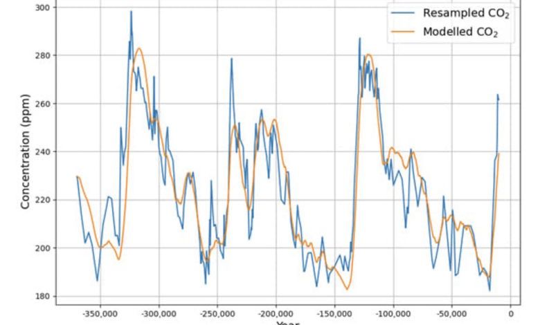
The corresponding estimated model results in a carbon sink effect of 1.3% of the concentration per century and a natural emission increase of 0.18 ppm per century from a 1 degree temperature increase. These are very small effects. Nevertheless, the reconstruction of CO₂ data from the temperature-extended sink model looks quite remarkable, as displayed in Figure 8.

Figure 8. Reconstruction of Vostok CO₂ concentration time series from temperature time series by means extended linear model.

The quality of reconstruction and the clear time-shift based error minimum are quite strong arguments for temperature changes being the cause of CO2 concentration changes rather than the other way round.  But even today ice core data are used to motivate high CO2 sensitivity of 5 degrees or more.

Even if we tentatively accept CO₂ being causal for temperature changes, the ice core argument has a big problem. Fact is, that the CO₂ concentration range of the ice core data is between 200 ppm and 280 ppm, i.e. the factor between the maximum and the minimum is approximately 1.4.   It is also a fact that since before the industrialization when concentration was 280 and today with a concentration of 420 ppm the factor is 1.5, and the temperature change is approximately 1.2 degrees. It is inconceivable therefore that such extreme temperature changes as between the ice ages were caused by such small CO₂ concentration changes. The high sensitivity argument based on ice cores is therefore disqualified.

Conclusions

The apparent inconsistency between the sensitivity of the sink effects to short term temperature variations but invariance with respect to temperature trends has been resolved by identifying the collinearity between temperature trends and CO₂ concentration. During the last 65 years the correlation between temperature and CO₂ concentration has been very high. Consequently, all temperature trend dependence has been attributed to CO₂ concentration in the original linear model. By evaluating the measured data with a model, where the residual temperature is added, the actual temperature dependence can be measured. By this procedure, the model is extended to become truly temperature-dependent. Further research is needed to validate the results of the extended model with other measurements.

The temperature-enhanced model also reproduces nicely the CO₂ concentrations of the Vostok ice core data series. As a side effect, this confirms that in paleo-climate data series, temperature leads CO₂ concentration.

With recent data, where there is a strong correlation between CO₂ concentration and temperature, the temperature trend dependence is balanced; therefore, we have to accept that currently the anthropogenic emissions are the main visible driver of atmospheric CO₂ concentration, while temperature effectively only adds some zero-mean variability.