by Robert Ellison
I don’t raise the alarm at all, but there are tipping points in the Earth system. Megafloods and megadroughts. Abrupt warming or cooling of many degrees C in years or decades. Glacials and interglacials. Solar energy driving patterns of planetary turbulence and an ice, cloud and biology response. These have always been with us. Our limited geophysical instrumental series reveal a variability that can’t be distinguished from anthropogenic warming effects (Koutsoyiannis 2020 ). So it’s happening but perhaps not quite the end of the world yet.
A tipping point is ‘the critical point in a situation, process, or system beyond which a significant and often unstoppable effect or change takes place’. (Merriam-Webster) Earth system state space is multi-dimensional. Not as many worlds or string theory dimensions but as fractionally dimensioned strange attractors in the state space. When a threshold is crossed the physical system responds with positive and negative feedbacks until settling into a new climate state as the perturbation damps out. In oceans and atmosphere hydrodynamics the rule is that big whirls have little whirls and little whirls have littler whirls and so on to viscosity. Friction turns kinetic energy to heat. But turbulent hydrodynamics says that the next tipping point – big or small – is not far away. Ice, cloud, hydrology and biology respond – occasionally dramatically. Perpetual perturbations are seen at scales of planetary waves to littler whirls.
From an important report by the U.S. National Academies (2013) Abrupt Impacts of Climate Change: Anticipating Surprises”
‘As recently as the 1980s, the typical view of major climate change was one of slow shifts, paced by the changes in solar energy that accompany predictable variations in Earth’s orbit around the sun over thousands to tens of thousands of years (Hays et al., 1976). While some early studies of rates of climate change, particularly during the last glacial period and the transition from glacial to interglacial climates, found large changes in apparently short periods of time (e.g., Coope et al., 1971), most of the paleoclimate records reaching back tens of thousands of years lacked the temporal resolution to resolve yearly to decadal changes. This situation began to change in the late 1980s as scientists began to examine events such as the climate transition that occurred at the end of the Younger Dryas about 12,000 years ago (e.g., Dansgaard et al., 1989) and the large swings in climate during the glacial period that have come to be termed “Dansgaard-Oescher events” (“D-O events;” named after two of the ice core scientists who first studied these phenomena using ice cores). At first these variations seemed to many to be too large and fast to be climatic changes, and it was only after they were found in several ice cores (e.g., Anklin et al., 1993; Grootes et al., 1993), and in many properties (e.g., Alley et al., 1993), including greenhouse gases (e.g., Severinghaus and Brook, 1999) that they became widely accepted as real.’
More recently, Tim Lenton et al. (2020) have written a paper: ‘The growing threat of abrupt and irreversible climate changes must compel political and economic action on emissions.’ –

Oceans and the hydrological cycle
A 1990 geography coursework reading list included ‘Fluvial geomorphology of Australia’. More particularly, a paper by Wayne Erskine and Robin Warner on flood and drought dominated regimes (FDR and DDR) set me wondering. Why for God’s sake are there multidecadal regimes and sudden shifts in eastern Australian rainfall? ENSO was clearly involved – but the PDO wasn’t described for nearly another decade.

The multi-decadal rainfall-runoff variability is the result of Pacific Ocean periodicity. Positive phases of the Interdecadal Pacific Oscillation (IPO) are drought years in Australia – negative phases bring cyclones, storms and flooding rains. And there is a flow threshold where streams change from a meandering to a braided form. Streams slowly revert to the meandering form in IPO positive regimes. Compare DDR and FDR??? with the IPO (Fig. 5) of Henley et al 2015. Note transition years. The pattern involves both the Pacific Decadal Oscillation (PDO) in the north – and the El Niño-Southern Oscillation (ENSO) – in the south. Warm or cool sea surfaces persist for a while and then shift. ENSO has a beat that shifted from 6-7 years to 2 to 5 years at the turn of the 1900’s – with more intense and frequent El Niño (Vance et 2012) – and has 20 to 30 year phases of persistent El Niño or La Niña states coherent with the PDO (e.g. Franks and Verdon 2006). With driving winds and currents split at the equator by the Coriolis force of a spinning planet. More flow in the Peru and California Currents shoals the thermocline and surging cold deep-water surfaces. Trade winds intensify pushing sun warmed water against Australia and Indonesia. More cold – and nutrient rich water surfaces in the east. Wind and current feedbacks kick up a notch. At some stage trade winds falter and water piled in the west surges east. The latest Pacific Ocean climate shift in 1998/2001 is linked to increased flow in the north (Di Lorenzo et al, 2008) and the south (Roemmich et al, 2007, Qiu, Bo et al 2006) Pacific Ocean gyres. Roemmich et al (2007) suggest that mid-latitude gyres in all of the oceans are influenced by decadal variability in the Southern and Northern Annular Modes (SAM and NAM respectively) as wind driven currents in baroclinic oceans (Sverdrup, 1947).
Is the beat of solar origin an effect on polar vortices? Are the 20 to 30 year Pacific state shifts an echo of the ~22 year Hale cycle? Will cold winters return with a less active sun? Gyre velocities are driven by the polar annular mode footprint. In theory solar magnetism or ultraviolet may trigger shifts in hydrodynamic state space. State space being the sum of physical states the planet can occupy within the laws of physics. It would explain synchronous north and south Pacific flows. There are climate limits that are found in paleo data. States persist while small changes in the system build instabilities that at last push the system past a threshold. That and/or a black swan event. Perturbations in ice, cloud and biology damp out until the next tipping point. States recur because the limits are physical – and hence the state space is ergodic. Limits of the past 2.6 million years seem most relevant – and I take no comfort from that.

Source: NASA

Source: Unknown
Low level marine boundary layer stratocumulus are seen off Peru. ‘The decks of low clouds 1000’s of km in scale reflect back to space a significant portion of the direct solar radiation and therefore dramatically increase the local albedo of areas otherwise characterized by dark oceans below.2,3 This cloud system has been shown to have two stable states: open and closed cells.’ (Koren et al 2017) It is an example of Rayleigh – Bénard convection in which cloud cells some 20 km in diameter form in the lower troposphere. Inside the cell water vapour condenses, droplets collide with condensation nuclei and it rains out from the centre. Faster over warmer oceans leaving a reduced domain albedo and a positive ocean heat feedback to multidecadal – and presumably longer – eastern Pacific SST change. Heat is gained or lost from the oceans as a subsystem shifts between warm and cool SST in the eastern Pacific. The Pacific has been – since the early 1900’s – in a millennially warm state (Vance et al 2013) warming the planet.
For this period, the observations show a trend in net downward radiation of 0.41 ± 0.22 W m−2 decade−1 that is the result of the sum of a 0.65 ± 0.17 W m−2 decade−1 trend in absorbed solar radiation (ASR) and a −0.24 ± 0.13 W m−2 decade−1 trend in downward radiation due to an increase in OLR… Most of the ASR trend is associated with cloud and surface albedo changes (Figure 2d), which account for 62% and 27% of the ASR trend, respectively.’ (Loeb et al 2021) Low level cloud is some 10% in the 70% odd total planetary cloud cover – according to a New Scientist reader. That changes dramatically in the tropical and subtropical eastern Pacific. My favorite future tipping point is in this cloud type at levels of CO2 in the atmosphere possible by the end of the century (Schneider et al 2018). If we burn all the fossil fuels. The last time CO2 was at such levels there were crocodiles in the Arctic circle.

Source: NASA Earth Observatory
The Moy et al 2002 ENSO proxy is based on the presence of more or less red sediment in a lake core. More sedimentation is associated with higher rainfall in El Niño conditions. It has continuous high-resolution coverage over 11,500 years. It shows periods of high and low El Niña intensity alternating with a period of about 2,000 years. There is the shift from La Niña dominance to El Niño dominance a little over 5,000 years ago that was a tipping point – and is associated with the drying of the Sahel. Note the bifurcation in the millennial band at that period. There is a period around 3,500 years ago of high El Niño intensity associated with the demise of Minoan civilisation (Tsonis 2010).

The time “series and wavelet power spectrum documenting changes in ENSO variability during the Holocene (a). Event time series created using the event model (see Methods), illustrating the number of events in 100-yr overlapping windows. The solid line denotes the minimum number of events in a 100-yr window needed to produce ENSO and variance. (b) Most recent 11,500 yr of the time series of red colour intensity. The absolute red colour intensity and the width of the individual laminae do not correspond to the intensity of the ENSO event. (c) Wavelet power spectrum calculated using the Morlet wavelet on the time series of red colour intensity (b). Variance in the wavelet power spectrum (colour scale) is plotted as a function of both time and period. Yellow and red regions indicate higher degrees of variance, and the black line surrounds regions of variance that exceed the 99.98% confidence level for a red noise process (at 4–8-yr period, the regions of significant variance are shown black rather than outlined). Variance below the dashed line has been reduced owing to the wavelet approaching the end of the finite time series. Horizontal lines indicate average timescale for the ENSO and millennial bands.” Christopher Moy et al, 2002, Variability of El Niño/Southern Oscillation activity at millennial timescales during the Holocene epoch
Is there an equilibrium up to 20,000 years before 1993 and then a shift to a cooler state punctuated by Dansgaard–Oeschger events that get more frequent and bigger as we go back through the last glacial interlude? It is followed by the Younger Dryas. Not slow insolation changes – but an ice dam bursting and freshening the Arctic. Slow changes build to a threshold and then feedbacks in a globally coupled system pop up. There is a pulse of solar activity somehow seemingly translating into large spikes of heat. Sea ice breaks off from the margins and drifts south. Thus there is high resolution data from sediment cores and a discovery of tipping points.

‘The temperature record from [3] and labelled D-O events 2 to 8 in blue from [4]. Low 10Be events 1 to 20 labelled in red. Note the 10Be scale is inverted. These low 10Be events would equate to an active solar magnetic field, shielding Earth from Galactic cosmic rays. It is possible that another 3 weak D-O events are present at 10Be events 7, 10 and 15.’ Source: Euan Mearns
A strong Atlantic meridional overturning circulation (AMOC) brings warm, salty water to the Arctic where it cools and sinks. Freshening of surface water changes the threshold at which water sinks. Less north Atlantic water is funnelled north cutting salt transport and feeding back into Arctic freshening. At low points in Milankovitch insolation ice sheets survive summer and self-feedback into monsters. The Arctic is about as warm and fresh as it can get. Milankovitch insolation is at a low point. Do the hydrodynamic math. ‘The Atlantic Meridional Overturning Circulation (AMOC), a major ocean current system transporting warm surface waters toward the northern Atlantic, has been suggested to exhibit two distinct modes of operation. A collapse from the current strong mode to the weak mode would have severe impacts on the global climate system and further multi-stable Earth system components. (Caesar et al, 2021)

‘Schematic of the major warm (red to yellow) and cold (blue to purple) water pathways in the North Atlantic subpolar gyre. Acronyms not in the text: Denmark Strait (DS); Faroe Bank Channel (FBC); East and West Greenland Currents (EGC, WGC); North Atlantic Current (NAC); DSO (Denmark Straits Overflow); ISO (Iceland-Scotland Overflow). Figure courtesy of H. Furey (WHOI).
Biosphere
I fell into tipping points – pun intended. I was rehabilitating a shallow coastal estuary – just salty enough to make a lake that smelled like rotten eggs. The catchment is heavily urbanised and industrialised since convicts first hauled coal out of the ground. I pulled on my waders and confidently stepped into Lake Illawarra to sink to my armpits in a morass of mud and slime. The engineering student with me was laughing uncontrollably. It is all parkland and water sports now. Much as I loved my lake – I had other lakes to worry about. All over the world shallow freshwater or brackish lakes were changing colour.
The culprit is phosphorus. It settles slowly with fine particles and organic detritus. With rainfall-runoff a pulse of organic and inorganic nutrients is delivered to waterways. In the normal course of things – oxygen penetrates lake sediments some 20 mm. In the oxic zone – most phosphorus is oxidised and insoluble. Some 5-15% is in reduced, soluble, bioavailable forms. There is a little phosphene gas entering the atmosphere. Below the oxic zone it is anoxic – organisms use crystal lattice bound oxygen leaving soluble phosphorus. Nitrogen is also stripped of oxygen and dissipates as N2 or NOx gases. When a pulse of nutrients arrives in a lake algae blooms. When that dies it settles on the bottom with the likewise dead herbivores that consumed it and their faeces. Decomposition at the bottom depletes oxygen in sediment sending accumulated and now bioavailable phosphorus into the water column. This favours nitrogen fixers like blue-green algae. Benthic vegetation is shaded out freeing benthic sediment. There is a state change that is difficult to reverse. In my lake the channel was dug out increasing tidal exchange. That will shoal in the nature of estuarine channels. And by running catchment drainage through sediment traps, vegetated channels and artificial wetlands.
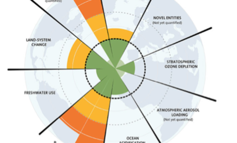
The biosphere is most obviously in trouble. It needs massive efforts by billions of people to manage forests, fisheries, aquifers, rangelands and waterways. And that takes peace, prosperity and a sense of humour. Fauna populations are crashing globally. The passenger pigeon’s survival strategy was sheer numbers. As people shot them out they crossed a threshold between recruitment and mortality and crashed to extinction. Nutrient exports from mines, farms and industrial and urban areas are land and water management fixes waiting to happen. Land and water management is our entire future. We have been losing carbon from agricultural soils and in traditional burning for 10,000 years. It is time to tip the balance back by managing for positive carbon, nutrient and water budgets on 5 billion hectares of private cropping and grazing land – for more production and less inputs in everything from permaculture food forests to industrial agriculture. To feed the world for another 10,000 years what we take from the Earth must be returned. It is simple accounting. Climate change means building massive factories churning out modular nuclear engines. I want a purple one. Land and water management include holding back water in sand dams, terraces and swales, replanting, changing grazing management, encouraging perennial vegetation cover, precise applications of chemicals and nutrients, cover crops… We need it to feed the world in the next 50 years.

Source: Stockholm Resilience Centre
By far the best thing to do is to better manage water and land. On 5 billion hectares of private cropping and grazing land and in global commons on which our lives depend. I am much encouraged by progress by small, medium and industrial farmers. To use plants to mine carbon from the sky and sock it away as organic matter in deep, rich, living soils. It reduces input costs – increases productivity – and feels socially good. Triple bottom line win win win – oi oi oi. Rattan Lal – doyen of soil science and 2021 winner of the World Food Prize – says that some 500 GtC (c.f. 350 GtC of modern anthropogenic emissions) has been lost from agricultural soils and in traditional burning over 10,000 years – a lot in the past 200. We should at least try to see how much can be restored this century – for biodiversity and food security. There is no plant carbon starvation at anywhere near today’s concentration.
The great global commons are best managed by local stakeholders with global information services. Big data can monitor most things. It is being used to predict the behaviour of complex ecological systems – e.g. Ye et al 2014. Cooperative polycentric management needs transparent data. Energy needs a powerful low-cost low-carbon source to meet rapid growth in demand. Modular nuclear engines rolling off assembly lines and onto trucks – or floating out of shipyards ready to connect – to meet an energy demand growth of 350% this century – is easily the frontrunner. There will be an energy transition – and because of course there are always creative/destructive tipping points in markets – the transition away from messy and bulky coal and gas will be rapid. I’d guess the lifetime of coal and gas plants being built now – if in future they can still find the parts.