Durham, NH
Executive Summary:
The recent UN report urgently calling for immediately disaster risk reduction measures is based on incorrect analysis and even simple computational errors.
A tool for analyzing nonlinear “kinks” in time-series data is developed and presented and used to identify “current trends” in disaster frequency that are very different from the long-term trends claimed by the United Nations Office for Disaster Risk Reduction.
Introduction:
Recently the United Nations Office for Disaster Risk Reduction issued a 256-page report subtitled, “Transforming Governance for a Resilient Future.” The report calls for immediate “rewiring” of multinational governance structures to prepare for a forecasted nearly “tripling of extreme weather events” between 2001 and 2030, and a rapid increase in general disasters globally, “from around 400 in 2015 to 560 per year by 2030.” The report lays out urgent measures to take to deal with these increasing disasters, calling for massive investment and international cooperation, along with rewriting rules by which we live.
The “Challenge” facing all of mankind is laid out in several key graphs, shown both in the paper and, in a more colorful form, on the UN website summarizing the paper. That is, the entire paper is based on the premise that disasters are increasing in frequency and severity, and mankind is at risk unless we take massive action to make preparations.
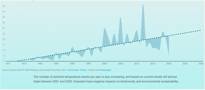
The foundational graph describing the problem is reproduced below, taken from the UN website.

As should be immediately apparent to any skilled data analyst, the least-squares linear regression presented does not represent the underlying data well. Specifically, the “error” in the graph (the deviation of the estimated value from the actual values) increases dramatically after the late 1990s. This indicates that linearity of the data breaks down sometime around the late 1990s, so forecasts based largely on earlier data become invalid.
Fortunately, the website includes a link to the data used to generate this rather alarming graph, allowing for independent analyses.
While it is tempting to draw a line from the data around 1998 diagonally downward and conclude “Disasters are actually becoming less common!” such an approach lacks rigor, and is as susceptible to the same type of sophomoric mistakes and biases that led to the creation of this graph. A more rigorous statistical approach is needed to determine when it is inappropriate to treat a data set as “linear,” and when it would be more appropriate to split the data set more than one line for estimation separately.
In response, I have created such a technique, which I term “kink analysis.” The kink analysis technique will be described in detail in the second half of this paper, and discussion regarding this tool (which is highly applicable to analyzing trends in climate data as well) is welcomed. The tool developed for the this “kink analysis” was then applied to the data presented by the UN to determine whether or not their application of linear regression to forecast future disaster rates was reasonable.
Kink Analysis Applied to the UN Disaster Data Set
Total Global Disasters
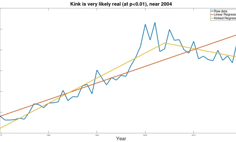
Applying the kink analysis tool (described in detail below) to the data on disasters from the UN report produced the following, with implications that are extremely dissimilar from the UN conclusions:

Here the blue line is the raw data, the brown line is the estimate from the UN, and yellow lines show the kinked trends implied by the data.
Statistically, the presence of the kink is extremely significant, at p<0.000005. The kink was found to exist somewhere near year 2004, but the confidence limits on the actual year of the kink are not yet defined (meaning that a search for the mechanism to explain this kink should be focused on a few years before or after 2004). Introduction of the kink reduces the pooled standard error by 58% vis-à-vis the standard error of the simple linear regression that appears in the UN report. The reduction of the standard error, paired with the statistical significance of the difference in slopes of the two lines (before and after the kink), indicate that the kinked model is far better at explaining the data than the linear model.
The most important finding here is that, in stark contrast to the claims by the UN report, frequency of disasters appears to be declining. While the UN report, based on their flawed application of a simple linear regression model claims ominously that “if current trends continue, the number of disasters per year globally may increase from around 400 in 2015 to 560 per year by 2030 – a projected increase of 40%,” the kink analysis indicates that current trend is quite different from what is presented, and disasters per year will most likely decrease to 158 per year, a decrease of more than 60%, back to the level of 1980. (While, of course, a declining trend cannot continue indefinitely, and at some point must slow and stop, the point remains that the alarmist UN claim regarding the “current trend” is completely misleading, and the panicked report demanding immediate action is wholly misguided.)
Occurrence of Drought
The UN report also forecasts expected drought by the year 2030, presenting the following chart, claiming that drought will be up “from an average of 16 drought events per year during 2001–2010 to 21 per year by 2030.”

The year to year variability is much higher in this data set, with some apparent cyclicality. Perhaps due to the greater variability, the kink analysis yields only slightly significant results, which are not to be trusted. I include the graph below just for the sake of completeness.
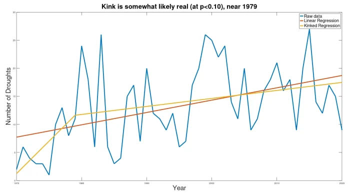
The results here are not substantially different from the results published by the UN.
Extreme Temperature Events
The UN report also includes a graph indicating increasing “extreme temperature events,” claiming that such events will “almost triple 2001 and 2030.” (It should be noted that, according to the UN data, while in 2001 the actual number of extreme temperature events was reportedly 23, they predict only 28 such events in 2030, an increase of only 13%. 13% is NOT “almost triple.” Even if we give the author the benefit of the doubt and note that the trend line was at 14 in 2001, still the predicted 28 events in 2030 cannot be termed “almost triple.” While the profusely illustrated report filled with charts and graphs causes one to believe the conclusions written in the report, simple arithmetic errors like this strain credibility.)
While the UN report shows a steadily rising trend, the kink analysis tells a very different story.
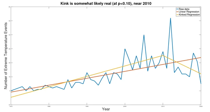
While the significance is only weak (at p=0.083, with a total reduction in pooled standard error of only 17.4% vis-à-vis the simple linear regression), again the “current trend” is downward, indicating the most likely future trend will be downward. Indeed, despite claiming that the number of extreme temperature events will triple between 2001 and 2030, in seven of the last eight years the number of extreme temperature events has been less than that of 2001 (averaging 36% fewer extreme temperature events than in 2001). While the downward trend found in the current data is not sustainable (as the projection of this trend to 2030 would result in a number less than zero), the statistics support a continued downward trend, so the best estimate for 2030 is not “tripling” the frequency from 2001, as claimed by the UN report, but rather a substantially lower frequency than the frequency in 2001.
Conclusion
The motivation for the UN’s urgent call to action is laid out on their web site that summarizes the “Transforming Governance for a Resilient Future” report. The motivation for calls for action is captured by the three graphs given above that the report claims to show increasingly frequent disasters that require that we change “governance systems” (including “reworking financial systems” to enable more governmental control). Fortunately, it appears as though the UN analyses of risk, based on their graphs, are completely incorrect. The urgency for dramatic action called for by this report is based entirely on analytical errors and even stark computational errors. Thus this UN report is not to be trusted, and must be dismissed. The lack of statistical (and even calculating) skills seen in this report calls into doubt other UN studies and statistical reports.
Part II
Kink Analysis
The basic question is this – is it possibly to rigorously identify whether or not there is a “kink” in a time-series data set (such as in the UN data presented above), along with the location of the kink. While often data analysts have “eye-balled” the existence of reversals of trends (in climate data, for example), for an analysis to be rigorous it must be objective, and thus subjective factors that sometimes reflect the biases of the analyst must be removed. Thus the question becomes that of, “Can a ‘kink’ in a time-series be identified through an objective statistical method?”
The technique set forth below was developed in response to this question:
- Assume that a change point (a “kink point”) may exist in the data set. For each point in the data set (termed a “candidate kink point”), split the data set at that point (with the candidate split point present in both data sets that are produced), and run regressions on the data before and after the candidate kink point, constraining the junction between the two line segments to be continuous. (In this paper, I use least-squares linear regression, using Octave, with some data transformations to ensure that the two line segments are continuous with each other.)
- For each candidate kink point, calculate the pooled estimation error for the entire data set. (Because each line segment includes the candidate kink point, the error at the candidate kink point itself is counted twice, providing a penalty for the use of this point, thereby preventing overfitting.)
- Select the candidate kink point that minimizes the total error. At this point, the amount of reduction in pooled estimation error (vis-à-vis a single linear regression) can be calculated easily, showing how the kinked-line model more closely matches the data set than a single linear regression.
- Use a t-test to calculate whether the two line segments have different slopes, and accept the candidate kink point as being an actual kink point if the t-test indicates that the difference in slopes of the line segments produced are statistically different.
Do this by finding the standard error in the estimate of each slope using the standard equation:

Then calculate the t statistic as follows, again using the well-known equation:

5. Check for two-tail significance of the t-statistic using degrees of freedom = total number of data points in the set minus 3. (Typically when comparing slopes of two lines one would consume 4 degrees of freedom in the lines, but the join is constrained to be continuous at the candidate point, so only 3 degrees of freedom are consumed.)
6. Accept the line is “kinked” if t-value is highly significant (p<0.01), consider that a kink may exist if the t-value is weakly significant (p<0.10), and reject the line being “kinked” otherwise.
I wrote an Octave/Matlab program to carry out the calculations described above, and tested it on simulated data sets of linear data with superimposed Gaussian noise. In 20 trials, the program produced results that would be expected, with one spurious kink found at the p=0.10 level, one spurious kink found at the p=0.05 level, and no spurious kinks found at the p=0.01 level.
Conversely, when simulated data sets with kinked signals with superimposed Gaussian noise were tested, the kinks were found with strong statistical significance despite substantial noise. Two examples are given below.
Example 1: Large Data Set (2000 points)
A signal as shown below was used as the foundation.
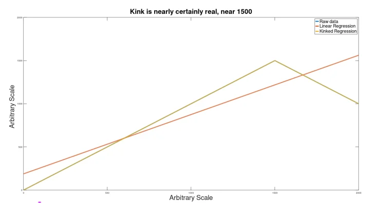
To this, a Gaussian noise signal was added, and the result was run through the kink analyzer to see if the signal would be found.
Despite the extreme noise, still the kink (which would actually be imperceptible to the eye) was discovered (at p=.005), to produce a kinked regression line closely matching the hidden input signal.

The location of the kink was somewhat incorrect (at 1550 instead of 1500).
With less noise, however, the location of the kink was identified more accurately.
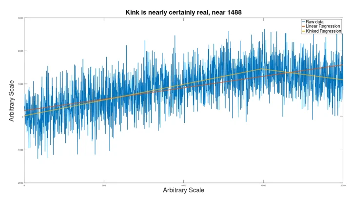
Here the existence of the kink is somewhat perceptible to the human eye, but completely beyond question statistically, with a p value of 7e-24.
Example 2: Smaller Data Set (200 Points)
On a similar kinked data set as used above, Gaussian noise was applied, followed by kink analysis. The result is shown below.
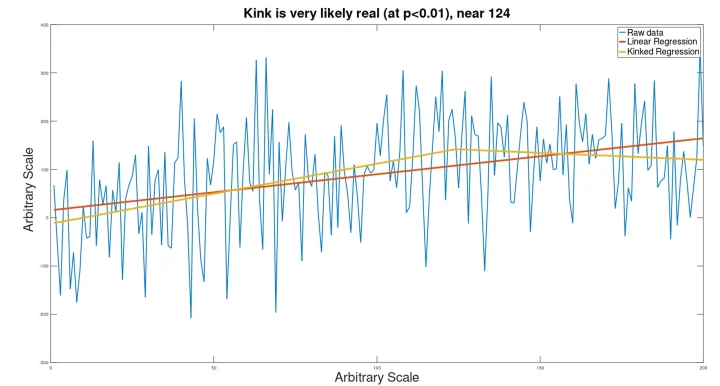
Although the kinked nature of this data set is not visible to the eye, the analysis was still able to identify that there was a kink (although it was calculated to be near point 124 instead of point 150).
With less noise, the location of the kink is identified more accurately.

Limitations:
This technique will identify a curved line (such as a logarithmic curve) as having a kink. Also, at this point I have no statistical method by which to place a confidence interval on the location of the kink.
Conclusion:
It is anticipated that this technique will be applied to policy analysis, looking for changes in trends in climatology, crime statistics, etc., where policy interventions and other factors cause trends to change over time (rendering simple linear regression inappropriate).