Guest Post by Willis Eschenbach
In my previous post, “Global scatter chart“, I discussed how to use a grid plot of the entire globe to better understand the relationship between two variables. The variables that I discussed in that post are the cloud radiation effect (CRE) as a function of temperature. At the end of that post, I threatened the following:
I will return to what I have learned from other gridcell scatterers in the next post.
So, as foretold in ancient texts… he is a fool!
For this exploration into global scatterplots, Figure 1 shows surface temperature as a function of the amount of solar electricity actually entering the climate system. This available solar energy is solar above the atmosphere (TOA), minus “albedo reflectance,” which is the amount of sunlight reflected back into space by clouds and surfaces.
Figure 1. Scatterplot, cellcell-by-gridcell surface temperature relative to available solar power. Number of grid cells = 64,800. The cyan/black line represents the LOWEST smoothness of the data. The slope of the cyan/black line shows the temperature change for each 1 W/m2 change in available solar energy. The data in all of these posts is an average of all 21 years of CERES data.
I mentioned before how I love the surprises science has to offer. What surprised me was that there are three very distinct modes shown in Figure 1.
The left side of the plot, under available solar about 100 W/m2, shows areas near the poles where there is very little solar power. In those areas, the temperature rises very quickly with the increase of solar power.
Then there is a basically long straight from ~100 W/m2 of available solar up to about 300 W/m2.
And finally, from about 310 W/m2 to 360 W/m2, there is a flat straight line, with no slope at all.
That was the biggest surprise for me. When the average solar available is above 310W/m2, you can add up to 50 W/m2 without raising the surface temperature a little. And remember, these are not short-term changes. This reflects the effect of the 50 W/m2 increase applied over decades and centuries.
Hmmm… an increase of 3.7 W/m2 from a doubling of CO2 is supposed to increase the temperature by 3°C. But this is the part of the world where the 50 W/m2 change is larger. ten times, no… nothing. However, I digress…
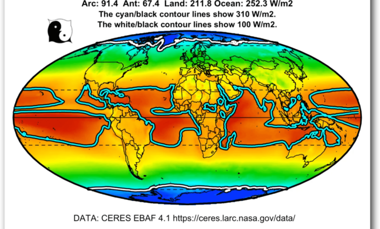
How does a large part of the world show this insensitivity? Figure 2 outlines areas below 100 W/m2, where there is a sharp increase in temperature as solar increases, and areas above 310 W/m2, where there is NO increase in temperature as solar increases.
Figure 2. Solar power available (solar TOA minus albedo reflectance), views centered on the Pacific Ocean and Greenwich. The areas outlined in red in cyan/black do not change in temperature as the average solar input increases. Polar regions in blue bordered by white/black indicate that the temperature is very sensitive to increased solar input. The horizontal lines represent the tropics and the arctic/antarctic circles.
Note that the red areas that are not sensitive to increased solar input are all in the tropics and are mostly oceanic. They cover half of the tropics or about 22% of the planet’s surface.
The blue regions, on the other hand, are sensitive to high temperatures for solar variations, covering only about 8% of the planet’s area.
Going back to Figure 1, recall that I said that “The slope of the cyan/black line shows the temperature change for each 1 W/m2 change in available solar energy.“Figure 3 shows exactly that, the slope of the cyan/black trendline in Figure 1.
Figure 3. Slope of the trend line in Figure 1. This shows the amount of temperature change for a 1 W/m2 change in available solar energy.
Here we see the same three regions we can see in Figure 1. On the left, under ~100 W/m2 of available solar, the sensitivity of temperature to changes in energy input the sun is quite high. (Remember, this is not climate sensitivity to CO2 changes. It is sensitivity to available solar energy.)
Then, from 100 W/m2 to 300 W/m2, the sensitivity is essentially unchanged, averaging 0.16°C per W/m2.
Finally, on ~310 W/m2 of available solar, the temperature is completely insensitive to changes in solar availability.
Note that this means that solar energy must increase by about six W/m2 to raise the temperature of 70% of the planet by 1°C… and remember that in half a tropical ocean, 22% of the planet, i.e. six W/m2 increase in available solar does not cause the temperature to rise. (“Doodly-squat”? It’s a techno-scientific term for zero.)
Inference? Homely.
An additional ~5 W/m2 solar input is required to raise the surface temperature by one degree Celsius.
Let me end with the threat from my previous post, viz:
I will leave this here, and I will return to what I have learned from other gridcell scatterers in the next post.
Best wishes to everyone on a foggy coastal day,
w.
I MEAN YOU: When you comment, quote the exact words you are responding. I can defend my word. I can’t defend your repeating my words. Thank.