Richard Willoughby
Summary
This technical note shows how the ocean surface temperature responds to the solar radiation at the top of the atmosphere. It highlights that the ocean surface is temperature constrained to the range -1.8C to 30C over a yearly cycle apart from less than 1% of the ocean surface near land masses in the tropics where the deep convection cycle is disrupted.
The atmosphere over oceans is dullest at 26C but the amount of reflective cloud increases above and below this temperature. At 30C, the reflected EMR achieves the level where just enough sunlight reaches the surface to evaporate the water required to power the deep convection engine driving global-scale air circulation. This precise temperature limit is similar to a speed governor on a reciprocating engine where the fuel supply is regulated to maintain engine speed. In the case of the oceans, the surface sunlight is the energy source that is being restricted by reflection from ever-brightening cloud with rising temperature from 26C until the 30C limit is reached.
The operation of the atmospheric heat engine is briefly explained with reference to the atmospheric temperature profile; referring to well-known meteorological phenomena such as Level of Free Convection and Convective Available Potential Energy. Those familiar with heat engines will draw analogies to the well-known Carnot cycle.
The factors causing climate change are discussed with reference to how the solar radiation is gradually changing over any point on Earth’s surface due to Earth’s orbital changes. The observed changes in temperature are the result of changing solar radiation at the top of the atmosphere except the Equator where the temperature has remained with no trend since satellites have been recording surface temperature over the past 40 years.
The actual temperature measurement in the Nino34 region in the tropical Pacific is compared with the output from climate models that all predicted warming where there has been none. No climate model has predicted the observed temperature trend in the important Nino34 region of the tropical Pacific. All have a warming trend where there has been a slight cooling trend observed.
Ocean Surface Temperature
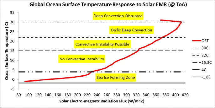
Global oceans have a near linear temperature response to solar electro-magnetic radiation (EMR) at the top of the atmosphere (ToA) averaged over an annual cycle with the exception of two clear inflection points and a third less distinct inflection point.
The distinct inflection points are at 4C and 30C. The less distinct point is at 26C where there is an increase in the slope from the near linear range between 4C and 26C.
The following image indicates the temperature distribution across the global oceans averaged over a yearly cycle.
From the image, the bright red areas are the only locations warmer than 30.5C. These are the locations where mid-level air divergence to land disrupts the normal deep convection over the oceans. The green regions are where sea ice forms and melts. Perennial sea ice is shown as grey as it responds to solar EMR in a similar way to land. The yellow hatched area in the central Pacific is known as the Nino34 region, which is used to forecast the different phases of the Pacific Ocean that influence global weather.
The inflection point at 30C is distinct and immutable with the present atmospheric mass. At 30C, the ocean heat engine literally runs out of steam due to persistent cloud formation. This can be observed globally by the reflection of the atmosphere in response to the surface temperature.
The most reflective white zones in the above image align with the bright red (>30.5C) zones in the temperature image. The inter-tropical convergence zone is also distinctive in the high reflective power near the Equator.
It is noticeable that the Southern Ocean is also highly reflective. This aligns with the surface temperature in the range -1.8C to 15C where convective instability cannot occur and some of the 15C to 22C where convective instability is not cyclic. The Southern Ocean and small regions in the North Pacific and North Atlantic have bright condensing/solidifying cloud due to air in circulation from low latitudes being cooled at higher latitudes.
The darkest, muddy yellow region of the reflection image broadly aligns with a temperature range from 24C to 27C where the ocean atmosphere is least reflective.
Deep Convection – The Heat Engine
The atmosphere over the oceans behaves as a self-governing heat engine. The Level of Free Convection (LFC) acts as the expansion nozzle between the high pressure and low pressure sides. The ocean surface is the evaporator and the atmosphere above the LFC is the condenser/solidifier. The formation of reflective cloud as the water vapour solidifies to highly reflective ice particles, limits heat input to the ocean by reducing surface insolation.
The following image examines the atmospheric isenthalpic lines for a surface temperature of 22C (295K), the lower limit of cyclic deep convection. It shows the moist isenthalpic line and the corresponding dry isenthalpic line through the LFC.
In this situation the LFC is at 2000m. The water vapour condensing zone below the 273K level will have 14.4mm equivalent of water vapour and the solidifying zone, where reflective ice cloud forms, will have 7.9mm. A complete cycle, under saturated conditions after cloudburst at 295K surface temperature, will have 40 hours of cloud forming and 35 hours clear sky or clear sky for 47% of the cycle. Normally instability occurs before the air above the LFC is completely dehumidified so cycles are shorter than 75 hours.
Here it is noted that moist air has lower density than dry air but there is a level of moisture where dry air will remain buoyant on moist air below. This is the altitude where the LFC forms. As the air above the LFC radiates energy to space, the water vapour above the LFC condenses or solidifies to cause the drying air to compress. The moist air below the LFC is more compressed than what it would be if free convection was not inhibited. The potential energy builds until the column becomes unstable giving rise to cloudburst. Cloudburst is the result of water vapour bursting into the dry zone due to the increasing buoyancy of the air as it becomes saturated. An analogy is that of a balloon bursting where compressed air suddenly expands once the balloon is punctured. The LFC is like the thin membrane of a balloon.
The profile of the atmosphere changes significantly when the surface temperature reaches its 30C (303K) limit.
The LFC in this condition is now much higher at 5600m. The moisture between the LFC and 273K is now only 7.4mm and the moisture above is 8.9mm. Under fully saturated conditions above the LFC, a full convective cycle will have 45 hours of cloud forming and just 8 hours clear sky. Without advection, the clear sky will persist for only 16% of the cycle time.
From observation at tropical moored buoys, the heat engine requires surface insolation averaging 200W/m^2 to keep the engine fully stoked. The drop in surface insolation with temperature is observed to be 20W/m^2/C. Pacific moored buoy 8N, 137E exhibited a trend of -21/2W/m^2/C for the six year period 2015 to 2020.
Atlantic moored buoy 4N, 23W exhibited -19.3W/m^2/C over the same period. The two charts use daily averages of one day for the Atlantic buoy and 5 day averages for the Pacific buoy. The thermal lag in the Pacific column averages around 25 days while the Atlantic, which is cooler on average, has much shorter response time of just 5 days.
From an energy balance perspective, it was observed that the convection column absorbs approximately 190W/m^2 of thermalised solar EMR in the column to drive the convection; most being in the form of sensible heat transfer to cooler regions. It only takes 11W/m^2 to extinguish the Convective Available Potential Energy (CAPE). The 30C column over open oceans always experience mid-level convergence and high level divergence. They are as powerful as the ocean atmosphere heat engine can get. CAPE in these systems is limited to about 3300J/kg; corresponding to peak updraft of 81m/s.
The Inter-Tropical Convergence Zone is dominated by these powerful convective towers that pump up the tropical atmosphere to drive global scale air and ocean circulations. They are responsible for distributing heat from the tropical oceans to the rest of the globe.
The Sun and Climate Change
Earth’s orbit around the sun is constantly changing. It is possible to determine the solar EMR available at the top of the atmosphere using orbital parameters and somewhat complex geometry.
The minimum average over the year 2021 was 170W/m^2 and the maximum average just over 417W/m^2 occurred immediately south of the Equator. Note that locations where sea ice exists can have lower annual average solar input than 170W/m^2 because the ocean water does not absorb sunlight when sea ice is present. This means the solar input to sea ice prone locations gets as low as 90W/m^2 over annual average.
The changes over time are relatively small and the best way of observing these changes is to consider the difference over a period. The following image indicates the change from 1982 to 2020 with 2020 having generally higher solar intensity.
If the sun was the sole driver of the ocean surface temperature then it would be expected to see reducing temperature in the high southern latitudes and increasing temperature elsewhere. Accordingly the NCEP Reynolds Optimally Interpolated SST data was used as basis for the following three charts.
So the Southern Ocean has cooled over the period as expected.
The mid-latitudes in the Northern Hemisphere have warmed as expected.
The equatorial zone, specifically the Nino34 region, has a slight cooling trend and does not respond to the increase in solar EMR intensity. This highlights the immutable limit of 30C on open ocean temperature.
It is also interesting to observe Jupiter’s beat (11.8 years) in this temperature record. Jupiter is so massive that it moves the sun slightly relative to other planets and that alters Earth’s orbit relative to the sun.
The performance of all climate models in the Nino34 region is poor. They all show warming trends in the region between 1980 and 2020 so do not even get the trend in the right direction. The following chart shows the output of the CSIRO Climate Model using the CMIP3 input data of early 2000s vintage.
Besides having the trend wrong, it also forecasts the physically impossible of the open ocean surface temperature sustaining 30C for months on this chart and permanently by 2100 in the model output. Climate models bear no relationship to reliable measured data.
The following chart shows the USA GISS (CMIP3) model forecast.
It also has an upward trend and forecast an average of 28.2C in 2022 where the observed average has been 27C.
The European MIROC (CMIP3) model also has a warming trend.
The average for 2022 is 25C, some 2C below the measured.
All the models have similar upward trends where there has been no trend while the predictions vary over a wide range, well outside any recorded temperature. The following chart compares the CMIP3 forecasts for the period 2020 to 2100.
The models all have an upward trend where none has yet been observed but the averages in 2020 vary from 24.5C for the MIROC model to 28.2C for the GISS model; almost 4C difference. The CSIRO is predicting sustained temperatures above 30C in this region but that cannot happen.
Simple Questions the Need Answers
Reliable temperature records show the global oceans are not undergoing universal warming. The ocean water in the mid northern latitudes is warming. The Equatorial oceans are showing no cooling or warning trend. The Southern Ocean is showing a sustained cooling trend. How can CO2 be selective in how it warms, cools or neither cools nor warms different locations on the globe?
Climate models are based on constant solar input. However the maximum solar intensity peaks when Earth is closest to the sun, currently in early January – 4th January in 2022. The timing of perihelion moves later, on average, by 13 days per thousand years. In 2104, perihelion will occur on the 7th of January for the first time this cycle. The distance from the sun at perihelion and aphelion also changes each year. Earth’s distance from the sun in 2020 averaged 18,000km less than it will in 2027. These small orbital changes influence the intensity of solar EMR. Why aren’t climate models using orbital changes to show both warming and cooling in response to the changing solar intensity?
Deep convection is a crucial atmospheric process that limits open ocean surface to 30C. How can climate models hope to reflect the real world when clouds are parameterised with no sensitivity to surface temperature?
Appendix
The image below is from the USA National Storm Prevention website. This shows the atmospheric profile in a skew-T plot from radiosonde sounding over Fort Worth/Dallas in June 2022. It includes values for CAPE and LFC among a number of other parameters used for storm prediction. It is similar to the simplified plots displayed above in this paper but the isotherms in the simple plots are shown vertically rather than skewed.
The rapid reduction in humidity above the LFC is the result of water vapour condensing/solidifying.
Data Sources
The data used to determine top of atmosphere reflected EMR were downloaded from NASA’s Earth Observation web site.
The data for climate models and NCEP measured SST were downloaded from the Climate Explorer website.
http://climexp.knmi.nl/start.cgi
The data for the moored buoys was downloaded from the NOAA PMEL website.
https://www.pmel.noaa.gov/tao/drupal/disdel/
The orbital parameters for determining the changes in ToA solar EMR came from the Astropicxels site:
Planetary Ephemeris Data (astropixels.com)
The image showing the Skew-T plot was downloaded from the USA National Storm Prevention website
https://www.spc.noaa.gov/exper/soundings/
The single column model (used to produce the atmospheric temperature profiles)is in the form of an Excel file with macro and is available by contacting the author using contact detail found at this link.
https://1drv.ms/u/s!Aq1iAj8Yo7jNhFRuXseL3rQ9SXoa
The Author
Richard Willoughby is a retired electrical engineer having worked in the Australian mining and mineral processing industry for 30 years with roles in large scale operations, corporate R&D and mine development. A further ten years was spent in the global insurance industry as an engineering risk consultant where he developed an enduring interest in natural catastrophes and changing climate.