Man-made CO2 and the expected results from its removal – Did it increase?

Clyde Spencer

2022

Introduce

This is a series of articles on the problem of man-made CO disposal₂; specifically why? no measurable deterioration in the atmosphere CO₂ occurred during the most severe reduction in anthropogenic emissions ever, during the shutdown of the 2020 SARS-Cov-2 pandemic.

I compare the measured CO₂ monthly emissions at Mauna Loa Observatory (MLO) with published figures for monthly anthropogenic emissions globally, for 2020, from the International Energy Agency (IEA) . Apparently, the IEA did not track anthropogenic emissions on a monthly basis, but only on an annual basis. However, it may be due to confusion and uncertainty as to why 2020 is compatible with the average global temperature of El Niño events of 2016, and there is no obvious decline in CO . year-on-year growth₂IEA decides to review monthly data.

I demonstrate that anthropogenic emissions are negligible compared to net CO₂ concentrations due to natural sources and sinks.

Analysis

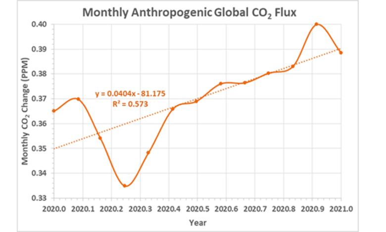
The analysis and conclusions depend on the following graphs, where all published ‘carbon’ mass units are converted to equivalent atmospheric CO Parts per million (PPM)₂ focus instead of using unfamiliar gigatons or petagrams. Figure 1, below, shows the shape of the curve obtained from the IEA monthly data, with the addition of a estimate for 2021 as a January ‘placeholder’. Note the minimum global value (-14.5%) As of April 2020. The IEA does not provide an estimate of monthly data uncertainty. However, according to Experimental rules in statistics, the standard deviation of man-made time series will be less than 1/4^order range, 0.065/4 or <0.02 PPM. The standard deviation of the anthropological series removing the trend would be around 0.041/4, or <0.01 PPM. That is, the trend accounts for about 0.01 PPM standard deviation for the year.

Figure 1. Monthly man-made CO2₂ line with trend line.

The slope of the OLS regression line, plotted but overshadowed by the data, for the monthly human-induced flux is statistically significant (p-value = 0.00272) at better than the 95% threshold , though, it only predicts a throughput gain of 0.04 PPM artificial CO₂ every month for more than a year. The OLS linear fit predicts about 57% of the variance between months, even with a significant, unusual drop in April.

Total monthly discharge for the 12 months of 2020 is 4.4 PPM, which is in line with other recent estimates of annual anthropogenic CO emissions.₂. That is, recent annual average human emissions up to ≈4.1 PPM (8.8 Pg * 1 PPM / 2.13 Pg) of 101 PPM total, or 4.1% of all sources.

The first thing a reader may notice is when the anthropological and net global data are combined (Figure 2, below), and scaled to show the full net global extent, the line The monthly birth rate is almost indistinguishable from a straight line. Man-made data has a near-constant flow of about 0.37 PPM CO₂ per month, for about 0.07 PPM CO₂.

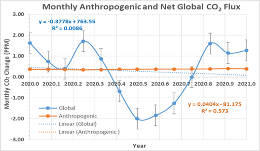
Figure 2. Monthly anthropogenic and global net CO emissions₂ throughput with each other.

Meanwhile, the monthly net global throughput is in a complex sinusoid, with a range of 3.71 PPM and a slightly negative trend (-0.38). However, this trend is not statistically significant (p-value = 0.763, R² = 0.0086) at the 95% threshold. The error bars included represent the mean (±0.5) standard deviation of the MLO measurements over this time period.

The obvious negative trend would not be surprising because, as pointed out by Moncton (2022), there was no statistically significant change in the Global Mean Temperature over 7 years. I used to prove a positive correlation between global temperature and the slope and extent of the seasonal increase in atmospheric CO₂. While correlation does not necessarily prove cause and effect, the association of increased CO₂ in warm times El Niño events imply that warmth is driving CO₂ because it is unlikely that the heat caused El Niño events! The important point is the seasonal net CO₂ range 57 times greater than that of man-made CO₂. That is, the annual range of anthropogenic emissions in 2020 is 1.8% of the seasonal real global range. That is Not drivers of annual changes; it’s ambient noise.

Man-made CO₂ Contributions have a range of almost an order of magnitude less than one sigma (1σ) uncertainty of the seasonal net MLO average, month-to-month measure change. Note in particular the relative position of the life line, during February, March, May and October in Figure 2, relative to the error bars. Even the nominal monthly mean human flux (0.37 PPM) is less than the monthly net global uncertainty. The anthropogenic contribution is a constant background component whose estimated monthly throughput is within the error range of the MLO change measurements.

Subtracting monthly anthropogenic emissions from monthly net global flows, as a first-order approximation, would shift the net global curve in Figure 2 by about 0.37 PPM, not change shape noticeably. NASA claim that “about 45 percent” of CO is caused by humans₂ emissions remain in the atmosphere. This is consistent with other claims that about half of anthropogenic emissions remain in the atmosphere. Based on that, to see what would happen if anthropogenic emissions stopped suddenly, we should subtract 0.17 PPM (45% of 0.37) from the monthly net global change stream . That’s much smaller than the 1σ uncertainty of monthly global net CO₂ flush.

When time series data are trending, it is common to observe false correlations between phenomena even when they do not have a causal relationship. It is usually encourage to de-trend the data and see if there is still a correlation. I do it below with this CO₂ data.

There is a negligible trend (slope = 0.04) in the anthropogenic data and a slope for net global CO₂ small enough (-0.38) that the appearance of the graph of the summation of residuals is essentially the same as in Figure 2; so I don’t show it. However, the net monthly change in global trends in 2020 is very similar in shape and magnitude to the NASA histogram (See Figure 3, below) for previous years of CO trend-reduced data. net monthly₂ change. Curve shapes have been surprisingly constant since at least 1959.

Figure 3. No-trend monthly atmospheric CO₂ throughput in PPM. (https://www.earthobservatory.nasa.gov/features/CarbonCycle)

However, it is advisable to look at the scatterplot of residual data without trending. Figure 4, below, shows that there are basically are not correlation between monthly anthropogenic emissions and net monthly global traffic; although the correlation is clearly negative, the regression line is Not statistically significant (p-value = 0.854) at the 95% threshold. CHEAP² values ​​show only 0.32% of variance in monthly net global CO₂ predicted or explained by monthly anthropogenic changes in emissions. In fact, the curves often go in different directions, like in April. (Compare Figure 1 and Figure 2 for April [2020.25]) If, there is any correlation, then the time lag might be obscuring it.

However, looking at the bigger picture, the year-on-year changes in anthropogenic emissions and the global net annual change in atmospheric CO2, there is little support. opinion that a lag time of more than one month is masking anthropogenic emissions control over total net source flux changes. Annual peaks in the northern hemisphere’s atmosphere₂ happened in May each five!

Similar to the analysis performed on the monthly residual data, Figure 5, (below) shows the trend disaggregated residuals graphed for cause and total annual net flow. Although there seems to be a slight positive correlation, it is not statistically significant (p-value = 0.943, R² = 0.0091). That is, the OLS regression line trend is so close to zero that it is statistically indistinguishable from the zero trend, and the squared correlation coefficient only predicts or explains about 0.91% of the variance in the net change between years.

Figure 4. Global correlation of monthly residual CO₂ change

for monthly anthropogenic CO residuals₂.

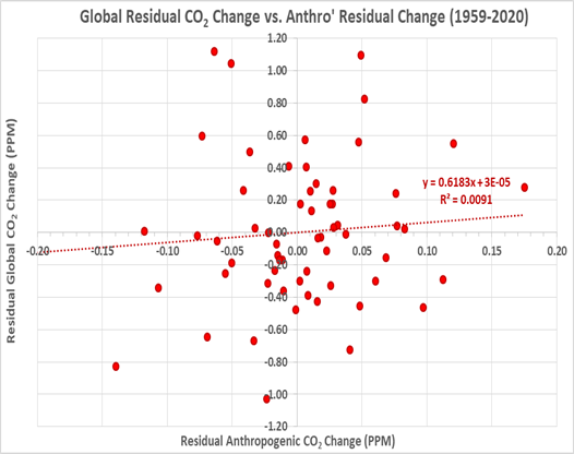
Figure 5. Global correlation of annual CO residuals₂ change

for annual anthropogenic CO residuals₂.

In brief

Man-made CO emissions₂ up to 4%, or less, of the total source throughput. The sinks are responsible for CO . extraction₂ from the atmosphere that are indistinguishable naturally from anthropogenic CO₂. Therefore, CO₂-source abundance determines the rate of rejection. Plant respiration and biodegradation govern the growth of the winter initiation stage; Photosynthesis prevails over Summer pull-down decline. That means man-made CO₂ does not accumulate at a nominal increase of 2 PPM per year. The annual increase in the global atmosphere is the increase from all source throughput, minus the attenuation of all sinks. CO caused by man every year₂ (0.07 PPM) in 2020 is only about 3.3% of the nominal 2 PPM annual increase. The monthly human-caused traffic is about 1.8% of the real monthly global throughput range. The fact that the 2 PPM annual increase in atmospheric emissions is about half of the estimated annual anthropogenic emissions is a coincidence. Perhaps those who see more things are expressing the common human trait adynamia. I am reminded of the great effort some people have put into finding special meaning in the measurements and ratios associated with Great Pyramid.

Man-made CO₂ virtually constant relative to the seasonal variation of natural sources and subduction. The monthly human-induced throughput change is much smaller than the uncertainty in the monthly net global throughput changes. Therefore, there is no support for anthropogenic CO claims₂ promote annual changes. Seasonal natural resources spill over to man-made sources. Eliminate man-made CO₂ would have a negligible impact on the annual increase, which is why pandemic shutdowns have had an imperceptible impact on global atmospheric concentrations. I don’t expect a drastic reduction of man-made CO₂ to have the kind of results claimed to justify phasing out fossil fuel use. Annual growth in CO₂ is the result of an increase in natural resources that is not offset by a commensurate increase in sinks.

Data sources

Dr. Pieter Tans, NOAA/GML (gml.noaa.gov/ccgg/trends/) and Dr. Ralph Keeling, Scripps Institution of Oceanography (scrippsco2.ucsd.edu/).

IEA (2021), Global Energy Assessment: CO2 Emissions in 2020, IEA, Paris https://www.iea.org/articles/global-energy-review-co2-emissions-in-2020

https://wattsupwiththat.com/2021/06/07/carbon-cycle/

https://wattsupwiththat.com/2021/06/11/contribution-of-anthropogenic-co2-emissions-to-changes-in-atmospheric-concentrations/

https://wattsupwiththat.com/2021/12/16/co2-party-having-fun-with-probabilities/