Into The Black Box – Rise to that?

Guest Post by Willis Eschenbach

Through what in my life has been a series of typical misunderstandings and coincidences, I ended up looking at the average model results from the Climate Intermodel Comparison Project 5 (CMIP5). I used the average of each model from each of the four scenarios, for a total of 38 results. The common time period for these results is 1860 to 2100 or some such number. I used the results from 1860 to 2020, so I could see how the patterns worked without looking at some imaginary future. The CMIP5 analysis was done a few years ago, so everything up to 2012 has actual data. So, 163 years from 1860 to 2012 is a “forecast” using actual forced data, and eight years from 2013 to 2020 is a forecast.

Figure 1. Model average CMIP5 scenario, plus overall average.

There are a few things I find interesting about Figure 1. The first is the massive virality. Starting from a common baseline, through 2020, model results range from 1°C warming up to 1.8°C warming…

With the terrible temperature spread between models forecast to 2012 plus 8 years forecast, why should anyone trust the models for what will happen in 2100?

The other thing that interests me is the yellow line, which reminds me of my post titled “Life is like a box of dark chocolate“. In that post, I discussed the idea of ​​”black box” analysis. The basic concept is that you have a black box with inputs and outputs, and your job is to figure out some procedure, simple or complex, to convert the input to output. In the present case, the “black box” is a climate model, the input of which is the annual “radiative emissions” from aerosols and CO₂ and volcanoes and things like that, and the output is the mean annual global temperature.

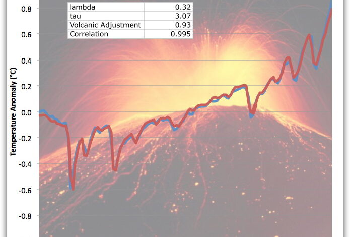
The same post also shows that the model outputs can be simulated in extremely high fidelity simply by reducing the delay and varying the input scaling. Here’s an example of how it works, from that post.

Figure 2. Original caption: “Functional equivalent equation of CCSM3 model, compared to actual CCSM3 output. The two are almost identical.”

So I’ve got a set of CMIP5 fortresses and used them to simulate averages of CMIP5 models (links to models and fortresses in Technical Notes at end). Figure 3 shows that result.

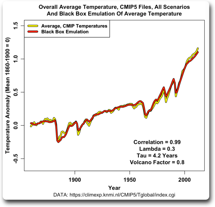
Figure 3. Average of CMIP5 files as shown in Figure 1, together with black box simulation.

Again it was a very close match. After seeing that, I wanted to look at some of the individual results. This is the first set.

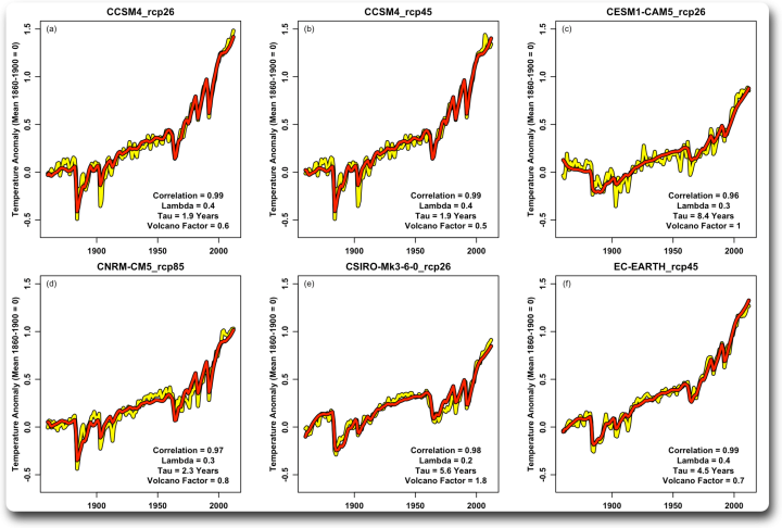
Figure 4. Six scenario averages from different models.

One interesting aspect of this is the variation in the volcanism factor. Models seem to treat stresses from short-term events such as volcanoes differently than a gradual increase in overall stress. And individual models vary, with pressures in this group ranging from 0.5 (applying half of the volcanism) to 1.8 (applying eighty percent additional volcanism) . The correlations are all quite high, ranging from 0.96 to 0.99. This is the second group.

Figure 5. Adding six scenario averages from different models.

Panel (a) at the top left is interesting, it is clear that volcanoes are not included in the compression for that model. Therefore, the volcanic coercivity is zero… and the correlation is still 0.98.

What this shows is that despite their incredible complexity and thousands upon thousands of lines of code and 20,000 2-D grid cells multiplied by 60 layers equates to 1.2 million 3-D grid cells… the output… Theirs can be simulated in a single line of code, viz:

BILLION_{(n + 1)} = TILLION_(n)+ F_{(n + 1)} / + T_(n) exp (-1 / )

OK, now unpack this equation in English. It looks complicated, but it’s not.

BILLION_(n) pronounced “T sub n”. It’s the temperature”BILLION“At time “n”. So, T by n plus one, is written as BILLION_{(n + 1)}, is the temperature for the following time period. In this case we are using years, so it will be next year’s temperature.

F is the radiative force from changes in volcanism, aerosols, CO₂and other factors, measured in watts per square meter (W/m²). This is the total of all the fortresses under consideration. The time convention is also followed, so F_(n) means to force”F“Period”n“.

Delta, or “Δ, means “change in”. So T_(n) is the change in temperature since the previous period, or BILLION_(n) minus the previous temperature BILLION_(n-1). Corresponding, F_(n) is the change in force since the previous period.

Lambda, or “λ, is the scale factor. Tau, or “τ, is the time delay constant. The time constant determines the delay in the system’s response to coercion. And finally, “exp (x)“Which means the number 2.71828 is a power of x.

So in English, this means next year’s temperature, or BILLION_{(n + 1)}equal to this year’s temperature, BILLION_(n)plus the immediate increase in temperature due to the change in forcing, F_{(n + 1)} /plus the deadline, T_(n) exp (-1 / ) from the previous coercion. This delay is necessary because the effects of changes in forcing are not instantaneous.

Curious, no? Millions of net cells, hundreds of thousands of lines of code, a supercomputer to crack them… and it turns out their output is nothing more than a delayed (tau) and scaled up version of the input (lambda).

Seeing that, I thought I’d use the same process on the actual temperature record. I used Berkeley Earth’s global mean surface air temperature record, although the results were very similar using other temperature data sets. Figure 6 shows that result.

Figure 6. Earth temperature record at Berkeley, and simulation using same compression as shown in previous figures. I have included Figure 3 on the right for comparison.

It turns out that the model mean is much more sensitive to volcanism, and has a shorter constant time tau. And of course, since the earth is a single example rather than an average, it contains more variation and therefore has a slightly lower correlation with the simulation (0.94 vs. 99).

So does this show that the fortress really controls the temperature? Well… no, for a simple reason. The forgings have been selected and refined over the years to be suitable for temperatures… so the fact that it does have no real value whatsoever.

One last thing we can do. IF the temperature is indeed the result of combustion, then we can use the above factors to estimate the long-term effect of a sudden doubling of CO₂ will. The IPCC says this will increase the force by 3.7 watts per square meter (W/m²). We simply use a step function to tie with a jump of 3.7 W/m² on a certain day. Here is the result, with a jump of 3.7 W/m² in the 1900 model year.

Figure 7. Long-term temperature change due to doubling of CO2₂using 3.7 W/m² as pressure increase and calculated with lambda and tau values ​​for Berkeley Earth and CMIP5 Model Average as shown in Figure 6.

Note that with a larger Tau time constant, the real earth (blue line) takes longer to reach equilibrium, on the order of 40 years, than using the mean of the CMIP5 model. And because real earth has a larger scale factor than Lambda, the end result is slightly larger.

So… is this the Equilibrium Climate Sensitivity Mystery (ECS) we read about so much? Dependent. IF forced values ​​are correct and IF forced temperature roolz … they are probably in the ballpark.

Or not. The climate is very complex. What I humbly call “Willis’s First Climate Law” says:

Everything in the climate is connected to everything else… which in turn is connected to everything else… except that it is not.

And now, me, I’ve spent all day washing the deck at the guesthouse, and my lower back is saying “LIE DOWN, FOOL!” … So I will leave you with my best wishes for a wonderful life in this endless mysterious universe.

w.

My usual: When you comment please quote exactly the words you are discussing. This avoids many of the misunderstandings that are the cause of intarwebs…

Technical Notes:

I have put all the modeled temperatures and tether data and a working example of how to do the adjustment as an Excel xlsx workbook in my Dropbox here.

Sources of Forcings: Miller et al.

The fortresses include:

• Well-mixed greenhouse gas
• Ozone
• Solar system
• Land use
• Snow Albedo & Black Carbon
• Trajectory
• Troposphere Aerosols Direct
• Troposphere Aerosols Indirect
• Stratospheric aerosols (from volcanic eruptions)

Model result source: KNMI

The average of the model situation used: (Not all model groups provide scenario averages)

CanESM2_rcp26
CanESM2_rcp45
CanESM2_rcp85
CCSM4_rcp26
CCSM4_rcp45
CCSM4_rcp60
CCSM4_rcp85
CESM1-CAM5_rcp26
CESM1-CAM5_rcp45
CESM1-CAM5_rcp60
CESM1-CAM5_rcp85
CNRM-CM5_rcp85
CSIRO-Mk3-6-0_rcp26
CSIRO-Mk3-6-0_rcp45
CSIRO-Mk3-6-0_rcp60
CSIRO-Mk3-6-0_rcp85
EC-EARTH_rcp26
EC-EARTH_rcp45
EC-EARTH_rcp85
FIO-ESM_rcp26
FIO-ESM_rcp45
FIO-ESM_rcp60
FIO-ESM_rcp85
HadGEM2-ES_rcp26
HadGEM2-ES_rcp45
HadGEM2-ES_rcp60
HadGEM2-ES_rcp85
IPSL-CM5A-LR_rcp26
IPSL-CM5A-LR_rcp45
IPSL-CM5A-LR_rcp85
MIROC5_rcp26
MIROC5_rcp45
MIROC5_rcp60
MIROC5_rcp85
MPI-ESM-LR_rcp26
MPI-ESM-LR_rcp45
MPI-ESM-LR_rcp85
MPI-ESM-MR_rcp45