Guest posts by Renee Hannon
This post evaluates the relationship of global CO2 with regional temperature trends during the Holocene interglacial period. Ice core profile shows CO2 is closely associated with local Antarctic temperatures and has been somewhat slow over the past 800,000 years (Luthi, 2008). While the emphasis is on CO2 and temperature lagging/conductivity, this study focuses on Holocene millennium trends in regions with different latitude limits.
Contrast Antarctica
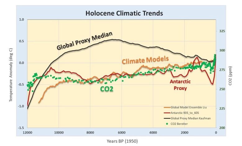
The Holocene is blessed with hundreds of proxy records analyzed by Marcot, 2013 and more recently Kaufman, 2020, to establish regional and global temperature trends. The Holocene Ice Age took place over the past 11,000 years. Collectively, global temperature trends from proxy data suggest a Holocene Climate Optimal (HCO) approximately 6000 to 8000 years ago and the subsequent cooling trend, the Neoglacial period, culminating in the Little Ice Age. (LIA). The global mean temperatures including regional trends with downward trends during the Holocene are shown in Figure 1a.
The exception is Antarctica shown in red with an upward concave shape. Antarctica reached an early Holocene climate optimum between 9000 and 11000 years ago. While global temperatures and most regions are warming, Antarctica cooled to a minimum around 8000 years ago. While the globe and other regions showed gradual cooling during the New Ice Age, Antarctica was flat and erratic. This contrasting Antarctic temperature behavior during the Holocene has also been documented by Andy May This.

Ice core temperature anomalies in Greenland and Antarctica derived from deuterium and/or oxygen isotopes and globally representative temperature vehicles are shown in Figure 1b. The long-term high resolution ice cores make them important proxy datasets. These data show similar trends with regional compilation. However, the temperature range tends to be larger at individual proxy sites. The smoothing of the paleoclimatic proxy data occurs by averaging multiple data types together, eliminating local temperature variation (Kaufman, 2023).
It’s not surprising that Antarctica’s temperature trends behave differently due to its unique environment. Antarctica is a continent surrounded by the Southern Ocean with an average annual interior temperature of -50 to -60 degrees Celsius. Most of Antarctica is covered by a permafrost with an average thickness of 2 kilometer. The sparse proxy data from Antarctica are mainly from ice cores and some marine sediments. These data include temperature trends in the 90oS-60oThe S latitude region represents less than 10% of the Earth’s surface area.
CO . gas2 nicely synchronized with the temperature in Antarctica
CO . gas2 Gas trapped in ice bubbles shows trends that are synchronous with local temperature anomalies in Antarctica during glacial and interglacial periods over the past 800,000 years. CO . gas2 ranges from a low of 180 ppm during the glacial period to a high of nearly 300 ppm during the glacial period. Figure 2a shows the linear regression of CO2 and temperatures from the EPICA Dome C ice core over the past 60,000 years, including the last glacial maximum and the Holocene interglacial. Regression squared (R2) is 0.9 which is very impressive. An interesting curiosity is the Holocene interglacial period where slopes tend to flatten out and2 significantly reduced to 0.3.
Although the correlation coefficient is lower for Holocene ice times, Figure 1a above shows CO2 shows concave trends such as temperature trends in Antarctica. CO . gas2 reached an early Holocene high near 275 ppm about 11,000 years ago after the ice melted. CO . gas2 then slowly decreased 10-15 ppm to a Holocene minimum of 260 ppm about 8000 years ago. And then, CO2 gradually increased to 290 ppm during the Neoglacial cooling period. It should be noted, these CO2 values are muted or smoothed due to gas trapping in the ice and do not reflect the values of the instrument (Joos, 2008).

Holocene CO . correlation diagram2 compared with the temperature anomaly from the high resolution regional proxy temperature shown in Fig. They are much different from the 60,000 year CO in Antarctica2 relationship in Figure 2a. Arctic and Northern Hemisphere regions (2c) show an inverse relationship with CO2, especially during the Neoglacial period. The tropics (2d) show a large dispersion with no statistically significant trends detected. Southern hemisphere, not shown, also has a low correlation with CO2. No other multi-regional or latitudinal temperature trends showed a strong positive correlation with CO2 in the Holocene like Antarctica.
The authors noted that CO2 trend is different from the global and Northern Hemisphere temperature trends. Vinos, 2022, concludes that CO2 runs counter to global temperature trends for most of the Holocene. This CO2 Asynchronous behavior and/or lack of correlation with temperature appear to be true for most regions, which cover about 90% of the Earth’s surface area.
Climate models dominated by forced CO2
Climate models that do not conform to representative global Holocene temperatures are known as the Holocene temperature conundrum (Liu, 2014). The models essentially show a gradual increase in temperature throughout the Holocene as shown in Figure 3a. Although temperature proxy data shows a Holocene Climate Optimal to be 0.5 degrees Celsius around 6000-8000 years ago, climate models simply do not reproduce.
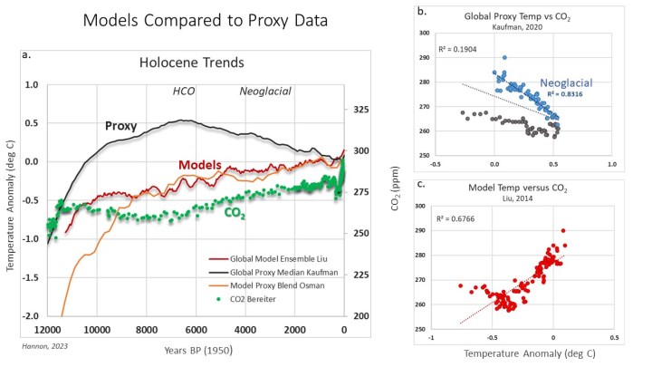
Holocene global proxy temperature trends show an inverse correlation with CO2 as shown in Figure 3b. There are two distinct inverse trends separated by HCO. During the New Ice Age, the representative temperature and CO2 shows a strong negative correlation with R2 of 0.8. Basically, like CO2 As global temperatures increase, global temperatures become colder.
Temperatures from model simulations are often controlled by changes in greenhouse gases, sunlight, ice sheets and freshwater flows, etc. The temperature profile is modeled in parallel with global CO.2 trend with a strong R2 of 0.7 confirmed CO2 is a main model control knob. In addition, the modeled Holocene temperatures tend to resemble opposite temperature trends in Antarctica (compare Figures 1a and 3a).
Scientists have begun to investigate the influence and ability of forces other than CO2. Zhang, 2022, modeled the effects of seasonal sun exposure and found a better agreement with proxy data when combining sunlight with ice sheet pressure, although not yet. perfect. Thompson, 2022, has shown that more vegetation influence in the Northern Hemisphere makes Holocene Optimal Climate simulation models clear in proxy data. The close relationship between CO2 and Antarctic temperatures suggest that millennium variations are strongly influenced by processes in the Southern Ocean. Only when past forces and their dominant times are more precisely incorporated into climate simulations will the models be able to predict future climate change.
observe
Climate change is often thought to be largely controlled by greenhouse gases, especially CO .2. This is partly concluded by the close relationship between CO2 from Antarctic ice core bubbles and Antarctic local temperature trends. While CO2 very well mimics Antarctic temperatures, 90% of the Earth’s surface temperature trends do not exhibit a positive correlation with CO2 during the Holocene. Temperatures in the Arctic and Northern Hemisphere become cooler as CO increases2 level. Tropical representative temperatures appear to be unaffected by CO2.
The simulated temperature model is strongly influenced by CO2 history does not exactly match global proxy temperatures during the Holocene and tends to largely reflect trends in Antarctica. The fact that CO2 correlates well with Holocene temperatures only in Antarctica, or <10% of our planet's surface, but CO2 considered the dominant influence on climate change is a scientific dilemma.
Download folder This.