Complexity of GMSL Measurement – Increasing with that?

By Andy May

Thomas Frederikse and colleagues published a study of sea level data that looked at both tide gauges and satellite data in 2020 (Frederikse, et al., 2020). This article is often cited in the discussion of sea level in Chapter 9 AR6. They found that there are many causes of global and regional sea level change that need to be considered. Soils across much of the Northern Hemisphere are still recovering from the melting of the giant glaciers they supported during the Last Glacial Maximum. This caused many tide gauges in the North to record a decrease in sea level as land rose. Furthermore, the construction of dams in the 20th century caused water to be trapped from the oceans and stored in reservoirs on land, especially between 1960 and 1980. They also tell us that the Previous assessments of sea level could not reconcile observations with the calculated contribution of ice. – mass loss, dam construction and thermal expansion of water. As mentioned in Part 1 of this series, the observed sea level change was very small, so this is not surprising. The annual changes are under the measurement accuracy of the instruments.

Observations of sea level, ocean temperature, loss of ice mass, water holdings in man-made reservoirs, and total river discharge into the ocean are all subject to considerable uncertainty, which is why why studies can’t close the gap between observations. Frederikse and colleagues make another attempt to close the gap. They note that over the past few years there have been more accurate estimates of all the important observations, and that they have collected these estimates in a new estimate.

Their best estimate of observed sea level rise trends from 1900 to 2018 was 1.56 ± 0.33 mm/year, ± 20% error. In Part 1 using NOAA sea level profile we obtain a slope of 1.74 mm/year, with R² 0.97, this value is within the 90% confidence limit given by Frederikse et al. The observed sea level change estimate is shown in dark blue in Figure 1. The sum of the sea level change components is shown in black. Two major components of sea level change are also shown for comparison. Static gas changes (ocean volume, excluding thermal expansion) are shown in red and temperature (change in ocean volume due to thermal expansion) are shown in orange. All curves focus on their 2002 to 2018 vehicles. Due mainly to the central period, the fit in the total composition and the sea level observations looks good for 21^st century. Before 1990, it wasn’t very good, but both the sum and the observations matched their respective margin of error. The observed sea level uncertainty, before 1990, usually exceeds ±10 mm; before 1960, it exceeded ±15 mm. Before 1940, it exceeded ±20 mm.

The sub-components of barystatic change studied in the paper are: melting of glaciers, melting of ice sheets in Greenland and Antarctica, and terrestrial water reserves (including building up) new dams and groundwater depletion). The heat change was estimated using measurements of subsurface ocean temperatures. Frederikse et al. tried to compare the total component with the observed sea level change as measured by satellite and tidal instruments using a model and found modest agreement, within the same margin of error. response.

The results of his study augment previous estimates of GMSL (global mean sea level) increases during the 1960s and 1970s, after excluding the effects of dam construction. His model also increased uncertainty before 1940. The coincidence was rather poor in the 1920s and 1930s, and sea levels rose between 1930 and 1950, almost as quickly as in the 21s.^st century, is also not a good fit.

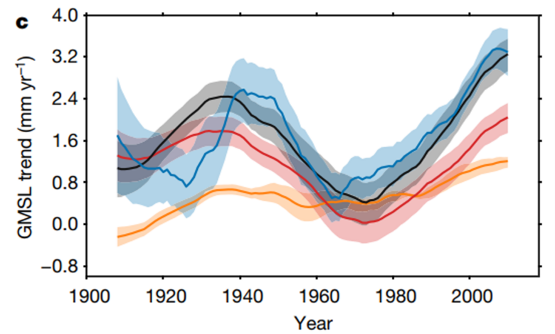
While uncertainty about the GMSL rate narrowed between 1993 and 2018, it still exceeded ±0.4 mm/year as shown in Figure 2. Both figures are part of Figure 1. Figure 1. 2 shows the 30-year interest rate of change against his model of calm and thermoregulatory change in red and orange, respectively, with their sum in black. They are compared with the rate of change observed over 30 years, shown in blue. It is clear that the rate of sea level rise fluctuates on a multilevel scale and could have increased as rapidly as it is today in the 1940s, within the margin of error.

In Figure 2, the shaded areas are 90% confidence intervals. The graph shows sea level rise rate in mm/year. The time periods where the match between the observations, in blue, and the model, in black did not match more clearly in Figure 2. The match was particularly poor between 1915 and 1950. The rate of increase slowed rapidly. from 1950 to 1965 is not a good fit at all. The rapid increase from 1990 to 2005 was only marginally better than in other periods.

Frederikse et al.’s model has a total uncertainty in the speed measurement of at least half a mm/year (see shaded in Figure 2) and uncertainty in the data (shaded in blue) even even bigger. Figure 2 is uncertain, but the 60-year oscillation is substantial and consistent with the normal long-term ocean oscillations described by Wyatt and Curry.^[1] Wyatt and Curry’s stadium waves can be seen in Figures 8 and 9 this. Their roughly 60-year cycle can be divided into a 30-year warming cycle and a 30-year cooling cycle. 1918 to 1942 was the warming period and 1942 to 1976 the cooling period in their analysis, which is quite consistent with the data shown in Figure 2.

Combining the Wyatt and Curry analysis with the analysis by Frederikse et al., we can see that the difference in sea level rise rates over 20^order in part probably the result of natural ocean oscillations. The Earth went into a natural warming mode in 1976, perhaps ending at the beginning of the 21st century, perhaps around 2005, and then into a deceleration mode. Judging from Figure 2, it appears that the apparent acceleration of sea level rise from the late 1980s to about 2005 is only a repeat of the acceleration from about 1925 to the early 1940s. Even if This is not true, it is clear that the data shown in Figures 1 and 2 are not accurate enough to conclude that the overall rate of sea level rise is increasing rapidly, in fact it is possible that we will see a deceleration of the sea level. sea ​​level. increase in the near future.

The statistical methods used in AR6 to show rather coarse sea-level rise acceleration, as discussed in Part 1. They simply picked the cherry data and used the smallest squares that fit them to estimate the acceleration. In this section, we show that the error in estimating sea level rise and its components is so large that a definitive representation of the acceleration is probably not possible. In the next article, we will discuss the problems with that approach and provide a clearer statistical forecast of sea level rise rates.

Folder can be downloaded this.

1. (Wyatt & Curry, The Role of Sea Ice on the Eurasian Arctic Shelf in a Hemisphere Climate Signal of Secular Change During the 20th Century, 2014) and (Wyatt, The “Stadium Wave”, 2014) ↑