Autocorrelation in CO2 and Temperature Time Series – Watts Up With That?

By Andy Could

In my last post I plotted the NASA CO₂ and the HadCRUT5 data from 1850 to 2020 and in contrast them. This was in response to a plot posted on twitter by Robert Rohde implying they correlated nicely. The 2 data seem to correlate as a result of the ensuing R² is 0.87. The least sq.’s perform used made the worldwide temperature anomaly a perform of the logarithm to the bottom 2 of the CO₂ focus (or ‘log₂CO₂‘). This implies the temperature change was assumed to be linear with the doubling of the CO₂ focus, a standard assumption. The least squares (or ‘LS’) methodology assumes there isn’t a error within the measurements of the CO₂ focus and all error ensuing from the correlation (the residuals) resides within the HadCRUT5 world common floor temperature estimates.

Within the feedback to the earlier put up, it grew to become clear that some readers understood the computed R² (usually known as the coefficient of willpower), from LS, was artificially inflated as a result of each X (log₂CO₂) and Y (HadCRUT5) have been autocorrelated and elevated with time. However a couple of didn’t perceive this important level. As most traders, engineers, and geoscientists know, two time collection which can be each autocorrelated and improve with time will virtually all the time have an inflated R². That is one kind of “spurious correlation.” In different phrases, the excessive R² doesn’t essentially imply the variables are associated to 1 one other. Autocorrelation is a giant deal in time collection evaluation and in local weather science, however too steadily ignored. To guage any correlation between CO₂ and HadCRUT5 we should search for autocorrelation results. Probably the most software used is the Durbin-Watson statistic.

The Durbin-Watson statistic exams the null speculation that the residuals from a LS regression will not be autocorrelated in opposition to the choice that they’re. The statistic is a quantity between 0 and 4, a worth of two signifies non-autocorrelation and a worth < 2 suggests constructive autocorrelation and a worth >2 suggests destructive autocorrelation. For the reason that computation of R² assumes that every commentary is impartial of the others, we hope that we get a worth of two, that means the R² is legitimate. If the regression residuals are autocorrelated and never random—that’s usually distributed concerning the imply—the R² is invalid and too excessive. Within the statistical program R, that is completed—utilizing a linear match—with just one assertion, as proven under:

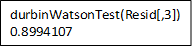
This R program reads within the HadCRUT5 anomalies and the log₂CO₂ values from 1850-2020 plotted in Determine 1, then masses the R library that comprises the durbinWatsonTest perform and runs the perform. I solely provide the perform with one argument, the output from the R linear regression perform lm. On this case we ask lm to compute a linear match of HadCRUT5, as a perform of log₂CO₂. The Durbin-Watson (DW) perform reads the lm output and computes the DW statistic of 0.8 from the residuals of the linear match by evaluating them to themselves with a lag of 1 yr.

The DW statistic is considerably lower than 2 suggesting constructive autocorrelation. The p worth is zero, which implies the null speculation that the HadCRUT5-log₂CO₂ linear match residuals will not be autocorrelated is fake. That’s, they’re seemingly autocorrelated. R makes it simple to do the calculation, however it’s unsatisfying since we don’t get a lot understanding from operating it or from the output. So, let’s do the identical calculation with Excel and undergo all of the gory particulars.

The Gory Particulars

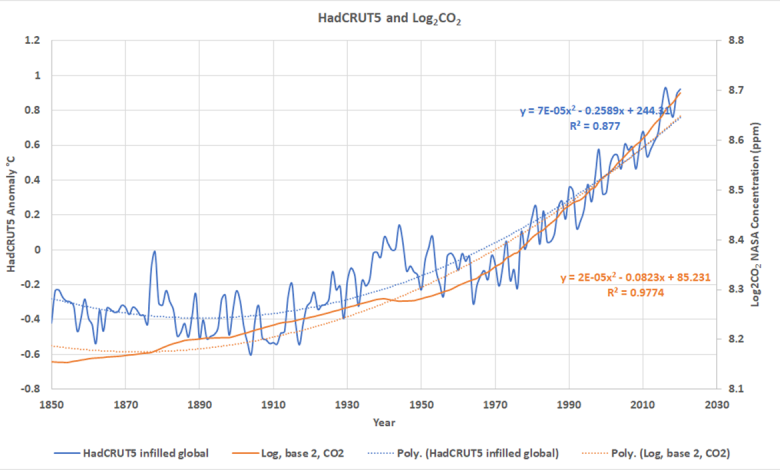
The fundamental information used is proven in Determine 1, it’s the identical as Determine 2 within the previous post.

Strictly talking, autocorrelation refers to how a time collection correlates with itself with a time lag. Visually we will see that each curves in Determine 1 are autocorrelated, like most instances collection. What this implies is that a big a part of every worth is set by its previous worth. Thus, the log₂CO₂ worth in 1980 may be very dependent upon the worth in 1979, and that is additionally true of the 1980 and 1979 values of HadCRUT5. This a crucial level since all LS suits assume that the observations used are impartial and that the residuals between the observations and the anticipated values are random and usually distributed. R² isn’t legitimate if the observations will not be impartial, a lack of independence shall be seen within the regression residuals. Under is a desk of autocorrelation coefficients for the curves in Determine 1 for time lags of 1 to eight years.

The autocorrelation values in Desk 1 are computed with the Excel components discovered here. The autocorrelation coefficients proven, like typical correlation coefficients, range from -1 (destructive correlation) to +1 (constructive correlation). As you possibly can see within the Desk each HadCRUT5 and log₂CO₂ are strongly positively autocorrelated, that’s they’re monotonically growing, as we will verify with a look at Determine 1. The autocorrelation decreases with growing lag, which is generally the case. All meaning is that this yr’s common temperature is extra intently associated to final yr’s temperature than the yr earlier than and so forth.

Row quantity one in all Desk 1 tells us that about 76% of every HadCRUT5 temperature and over 90% of every NASA CO₂ focus are dependent upon the earlier yr’s worth. Thus, in each instances, every yearly worth isn’t impartial.

Whereas the numbers given above apply to the person curves in Determine 1, autocorrelation can clearly have an effect on the regression statistics when the temperature and CO₂ curves are regressed in opposition to each other. This bivariate autocorrelation is normally examined utilizing the Durbin-Watson statistic talked about above, and named for James Durbin and Geoffrey Watson.

Linear match


As I did within the R program above, historically the Durbin-Watson calculation is carried out on a linear regression of the 2 variables of curiosity. Determine 2 is like Determine 1, however we have now match LS traces to each HadCRUT5 and Log₂CO₂.

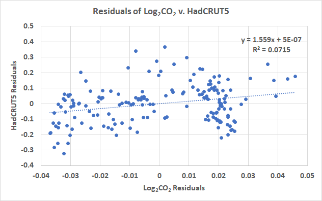
In Determine 2, orange is log₂CO₂ and blue is HadCRUT5. The residuals are proven in Determine 3, discover they aren’t random and seem to autocorrelate as we might anticipate from the statistics given in Desk 1. They’re autocorrelated and have the identical form, which is worrying.

The following step within the DW course of is to derive a LS match to the residuals proven in Determine 3, that is completed in Determine 4.

Simply as we feared, the residuals correlate and have a constructive slope. Doing the DW calculations on this trend, we get a DW statistic of 0.84, near the worth computed in R, however not precisely the identical. I believe that it’s because the a number of sum-of-squares computations over 170 years of information results in the refined distinction of 0.04. We will verify this by performing the R calculation utilizing the Excel residuals:

This confirms that each calculations match, however there have been variations within the sum-of-squares calculations as a result of totally different laptop floating-point precision utilized in Excel and R. So, with a linear match to each HadCRUT5 and log₂CO₂, there are critical autocorrelation issues. However each are concave upwards patterns, what if we used an LS match that’s extra acceptable {that a} line? The plots seem like a second order polynomial, let’s attempt that.

Polynomial Match


Determine 5 reveals the identical information as in Determine 1, however we have now match 2^nd order polynomials to every of the curves. The CO₂ and HadCRUT5 information curve upward, so it is a huge enchancment over the linear suits above.

I ought to point out that I didn’t use the equations on the plot for the calculations, I did a separate match to a long time. The a long time have been calculated utilizing 1850 as zero and 1850 to 1860 as decimal a long time and so forth to 2020 in order that the X variable within the calculation had smaller values within the sum of squares calculations. That is to get across the Excel laptop floating-point precision downside already talked about.

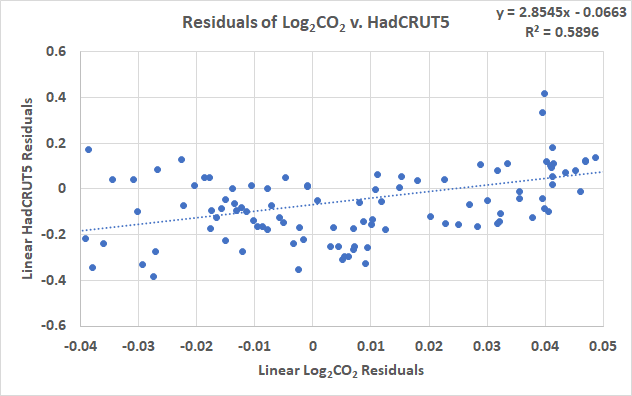
The following step within the course of is to subtract the anticipated or pattern worth for every year from the precise worth to create residuals. That is completed for each curves, the residuals are plotted in Determine 6.

Determine 6 reveals us that the residuals of the polynomial suits to HadCRUT5 and log₂CO₂ nonetheless have construction and the construction visually correlates, not a very good signal. That is the portion of the correlation left, after the two^nd order match is eliminated. In Determine 7 I match a linear pattern to the residuals. The R² is lower than in Determine 4

There may be nonetheless a sign within the information. It’s constructive, suggesting that if the autocorrelation have been really eliminated with the two^nd order match (we can’t say that statistically, however “what if”), there may be nonetheless a small constructive change in temperature, as CO₂ will increase. Bear in mind, autocorrelation doesn’t say there isn’t a correlation, it simply invalidates the correlation statistics. If temperature is generally dependent upon the earlier yr’s temperature, and we will efficiently take away that affect, what stays is the actual dependency of temperature on CO₂. Sadly, we will by no means ensure we eliminated the autocorrelation and may solely speculate that Determine 7 would be the true dependency between temperature and CO₂.

The Durbin-Watson statistic


Now the calculations to compute the Durbin-Watson joint autocorrelation are completed, however this time we used a 2^nd order polynomial regression. Under is a desk exhibiting the Durbin-Watson statistic between HadCRUT5 and log₂CO₂ for a lag of 1 yr. The calculations have been completed utilizing the process described here.

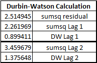
The Durbin-Watson worth of 0.9, for a one-year lag, confirms what we noticed visually in Figures 5 and 6. The residuals are nonetheless autocorrelated, even after eradicating the second order pattern. The remaining correlation is constructive, as we might anticipate, presumably which means that CO₂ has some small affect on temperature. We will verify this calculation in R:

Dialogue


The R² that outcomes from a LS match of CO₂ focus and world common temperatures is artificially inflated as a result of each CO₂ and temperature are autocorrelated time collection that improve with time. Thus, on this case, R² is an inappropriate statistic. R² assumes that every commentary is impartial and we discover that 76% of every yr’s common world temperature is set by the earlier yr’s temperature, leaving little to be influenced by CO₂. Additional, 90% of every yr’s CO₂ measurement is set by the earlier yr’s worth.

I concluded that one of the best perform for eradicating the autocorrelation was a 2^nd order polynomial, however even when this pattern is eliminated, the residuals are nonetheless autocorrelated and the null speculation that they weren’t needed to be rejected. It’s disappointing that Robert Rohde, a PhD, would ship out a plot of a correlation of CO₂ and world common temperature implying that the correlation between them was significant with out additional clarification (as we confirmed in Determine 1 of the previous post) however he did.

Jamal Munshi did the same evaluation to ours in a paper in 2018 (Munshi, 2018). He notes that the consensus concept that growing emissions of CO₂ trigger warming, and that the warming is linear with the doubling of CO₂ (Log base 2) is a testable speculation. This speculation has not examined nicely as a result of the uncertainty within the estimate of the warming as a consequence of CO₂ (local weather sensitivity) has remained stubbornly massive for over forty years, principally ±50%. This has precipitated the consensus to try to transfer away from local weather sensitivity towards comparisons of warming to combination carbon dioxide emissions, pondering they’ll get a narrower and extra legitimate correlation with warming. Munshi continues:

“This state of affairs in local weather sensitivity analysis is probably going the results of inadequate statistical rigor within the analysis methodologies utilized. This work demonstrates spurious proportionalities in time collection information that will yield local weather sensitivities that don’t have any interpretation. … [Munshi’s] outcomes indicate that the massive variety of local weather sensitivities reported within the literature are prone to be principally spurious. … Enough statistical self-discipline is prone to settle the … local weather sensitivity subject by hook or by crook, both to find out its hitherto elusive worth or to display that the assumed relationships don’t exist within the information.”

(Munshi, 2018)

Whereas we used CO₂ focus on this put up, many within the “consensus” are actually utilizing whole fossil gas emissions of their work, pondering that it’s a extra statistically legitimate amount to match to temperature. It isn’t, the issues stay, and in some methods are worse, as defined by Munshi in a separate paper (Munshi, 2018b). I agree with Munshi that statistical rigor is sorely missing within the local weather group. The group all too usually use statistics to obscure their lack of information and statistical significance, reasonably than to tell.

The R code and Excel spreadsheet used to carry out all of the calculations on this put up will be downloaded here.

Key phrases: Durbin-Watson, R, autocorrelation, spurious correlation

Munshi, J. (2018). The Charney Sensitivity of Homicides to Atmospheric CO₂: A Parody. SSRN. Retrieved from https://papers.ssrn.com/sol3/papers.cfm?abstract_id=3162520


Munshi, J. (2018b). From Equilibrium Local weather Sensitivity to Carbon Local weather Response. SSRN. Retrieved from https://papers.ssrn.com/sol3/papers.cfm?abstract_id=3142525