Lots of pressure to post this early and this morning it was raining in The Woodlands, so no golfing. I checked it again and think it’s fine. Here you are!
By Andy May
In Part 1 of this series, we examined the data and analysis presented in AR6 to support their conclusion that sea levels are rising rapidly. In Part 2 we have looked at a rigorous examination of the observed record of sea level rise over the past 120 years and the modeled components of that rise. We ended up in Part 1 that the statistical evidence presented in AR6 for acceleration is crude and selective. In Part 2 we find that the error in both the estimate of sea level rise and the estimate of the components of that increase is very large. The error ruled out the ability to determine the acceleration with any confidence, but the data revealed approximately 60-year fluctuations in sea-level rise rates consistent with known natural ocean cycles.
Modern statistical tools allow us to forecast changes in time series, such as GMSL (global mean sea level), in a more valid and sophisticated way than simple comparisons with squares The smallest is chosen as cherry as IPCC implemented in AR6. Our forecast is based on pure statistics. It’s done in a way that’s correct, but not necessarily, statistics are. We won’t know for sure until 2100. That said, let’s do it. If you have a certain type of nerd mind, you will love this.
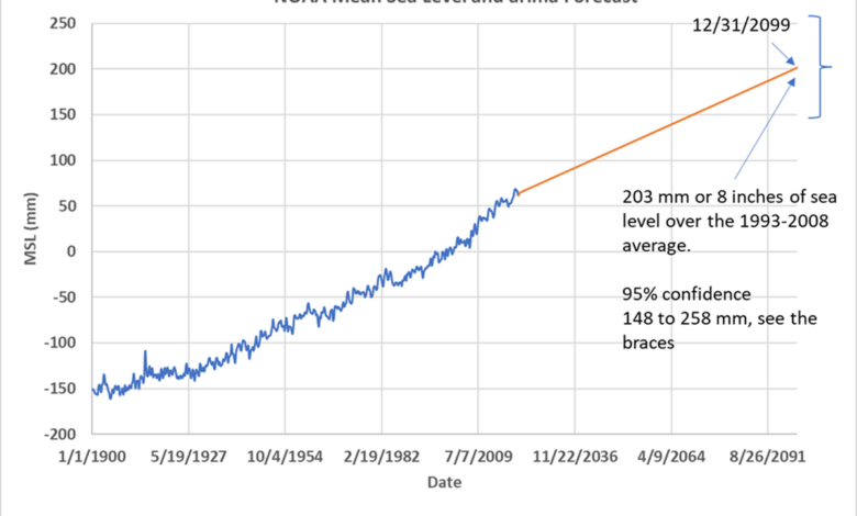
Figure 1 is the data plot we’ll be using — NOAA’s sea level dataset. Just by looking at it, we can tell it is autocorrelation, which means that the average sea level estimate for each quarter is highly dependent on the previous quarter’s value. Autocorrelation is important to consider in least squares regression, especially when forecasting time series, but is often overlooked by IPCC.

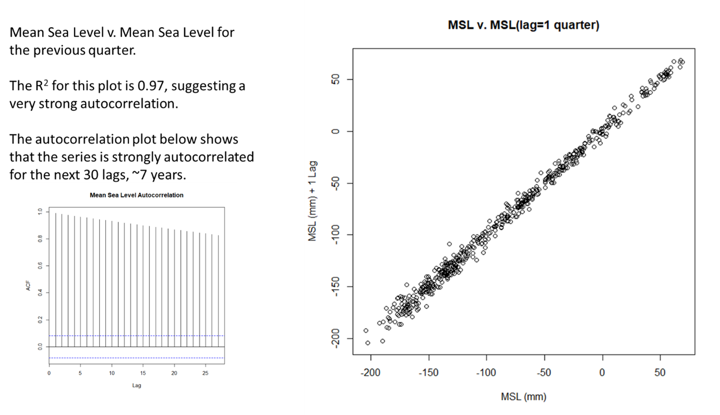
Figure 2 plots each sea level estimate against the previous one, this is called the histogram of the first lag, and the correlation of the two is a measure of autocorrelation. CHEAP2 of the first lag is 0.97, so sea level is very autocorrelated. This is obvious but means that the normal least squares linear fit statistic is not valid, the least squares statistic, such as R2assuming that The error of the regression is independent. The smallest square, as used in AR6 to display the acceleration, is not suitable for a dataset like this. Almost any given value is highly dependent on the previous value. This means that the mean square error (MSE) will be too small, making the error of the fit too small. As a result, any least squares line of the data in Figure 1 or any portion of that data is statistically useless, unless autocorrelation is calculated.
So how can we predict GMSL statistically valid? Obviously we cannot use least squares and need to apply more advanced techniques. The first step is to remove autocorrelation from the data, this is usually done by subtracting the previous GMSL value from the current value and progressing this way throughout the data set. We’ve taken this and show a histogram of the results in Figure 3.

The first difference data from GMSL looks pretty good, very much like white noise. This is exactly what we want for valid statistical analysis and forecasting. We will use a CHEAP function called “arima” to generate our GMSL forecast and this function requires three parameters to work, they are called p, d and q. These parameters tell arima how to condition the input data and build a model that can project valid values in the future. The graph in Figure 3 shows us that “d” is one. That means taking a difference of adjacent values will eliminate autocorrelation. We also need data to freeze, which are statistical properties that do not change over time (from left to right). The initial data set (Figure 1) is clearly not fixed, and that’s okay, we don’t want the way the GMSL changes to be a function of time for this analysis. The CHEAP Enhanced Dickey-Fuller test (ADF) function confirms this, since the original dataset has ADF p . value 0.79, which means it is not stationary. The arima p-value is not the same as the statistical p-test.
The difference plotted in Figure 3 has an ADF p-value of 0.01, which is lower than 0.05, the threshold needed to represent stability. The data are fixed when the distribution over the time period being studied is evenly distributed around the mean. That’s the distribution, up and down, that doesn’t change significantly over the time (x) axis.
Next, we need to infer the arima p and q values. To do this, we need the ACF (autocorrelation) and PACF (partial autocorrelation) graphs shown in Figure 4.
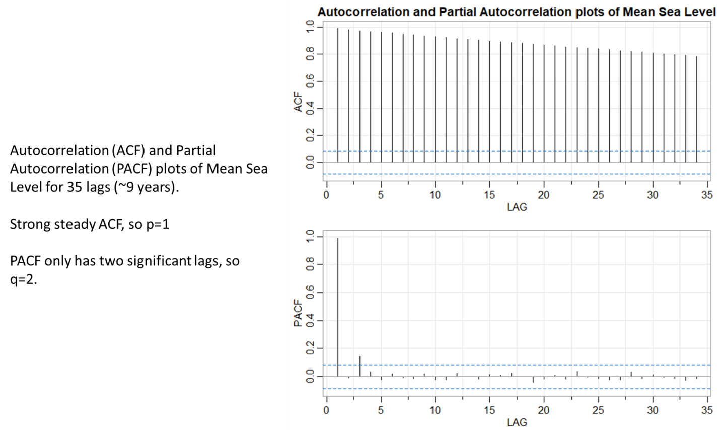
GMSL time series analysis gives us a arima parameter set of (1,1,2) for (p, d, q). We can also run an R function called auto.arima to see what parameters it recommends. We find that it is also stable on (1,1,2). This is good confirmation that our parameter choice was correct. Figure 5 plots the results.

Figure 5 tells us that the model is successfully capturing the nature of mean sea level trends from 1880 to 2020. The residuals of the model show no trends and they do not correlate with together. Figure 6 shows the arima forecast from the model (1,1,2).

Figure 7 is a diagram of forecast from Excel easier to read. The forecast we created predicts that GMSL will grow from 148 (6 inches) to 258 mm (10 inches) by 2100. Many researchers call this alarmingbut humans have successfully adapted to much higher rates of sea level rise in the past as we can see in Figure 2 of Post 1and they did so without the technology that we have today. When we consider the average open ocean daily tidal range of 1,000 millimeters or 3 feet, a sea level rise of 8 inches over 100 years doesn’t seem like much. In the 20th century, sea level rise 5.5 inchesDoes anyone notice or care, other than a few researchers?

Conclude
In the US, we call the AR6 effort to convince us that the GMSL increase is accelerating, using adjacent cherry-picked least squares lines as “high schools”, that is, uncomplicated. complex. Their method is problematic because GMSL is highly autocorrelated and non-stationary, showing their cherry-picked smallest squares fit and the least squares statistic invalid.
Our fit, using the R arima function, is at least statistically valid. We specifically fixed the autocorrelation and forced the series to stand still. We also deal with residual partial autocorrelation at the one-quarter and three-quarter level. The rest of our model surpassed the overall Check out Ljung-Box and multi-latency Ljung-Box tests for white noise, meaning that the arima model correctly captured a 140-year trend in NOAA sea level data.
Thus, while the periods were chosen by AR6 to support their conclusion that GMSL is accelerating, we reached the opposite conclusion using all data in a statistically valid manner. This does not mean that our forecast is correct, but it does mean that the AR6 speculation that sea levels could rise by 5 meters by 2150 is extremely unlikely and is best characterized as speculation. irresponsible. Our analysis found no statistical evidence of acceleration and produced a linear extrapolation.
While the warming of the Earth’s surface is clearly the reason for the melting of land-based glaciers, which contribute to sea level rise, AR6 offers no evidence that the warming is due to other activities. human movement. They use models to infer that humans caused it, but unfortunately their models are also not statistically valid as shown in Fig. Part 2, thisand by McKitrick and Christy (McKitrick & Christy, 2018). We can all agree that humans can have some effect on atmospheric warming, but we don’t know how much is man-made and how much is natural, because we We are rising from the unnatural cold. Little Ice Age– the “pre-industrial” period. Furthermore, as we have seen in Part 2, the rate of sea level rise in 30 years shows a clear natural fluctuation. Glacial ice and melting ice may be responsible for most of the sea level rise, as AR6 highlights, but the human share of that warming is likely to be quite small.
Thus, from a purely statistical point of view, the AR6 statements are childishly invalid. Proper data analysis leads to a forecast of about 20 cm (~8 inches) sea level rise by 2100. By 2100, our descendants will know who is right.
The R data and code for creating the figures in this chapter can be downloaded this. The R code and spreadsheet provide more detail on the arima forecast, including references not provided below.
McKitrick, R., & Christy, J. (2018, July 6). Testing the Tropical 200 to 300 hPa Warming Rate in Climate Modeling, Earth Science and Space. Earth and Space Science, 5(9), 529-536. Taken from https://agupubs.onlinelibrary.wiley.com/doi/full/10.1029/2018EA000401